Thesis Navigation
Cite as: Davis, Daniel. 2013. “Modelled on Software Engineering: Flexible Parametric Models in the Practice of Architecture.” PhD dissertation, RMIT University.
5.0 – Case A: Logic Programming
Project: Realignment of the Sagrada Família frontons.
Location: Barcelona, Spain.
Project participants: Daniel Davis, Mark Burry, and the Basílica i Temple Expiatori de la Sagrada Família design office.
Related publication: Davis, Burry, and Burry, 2011c.
5.1 – Introduction
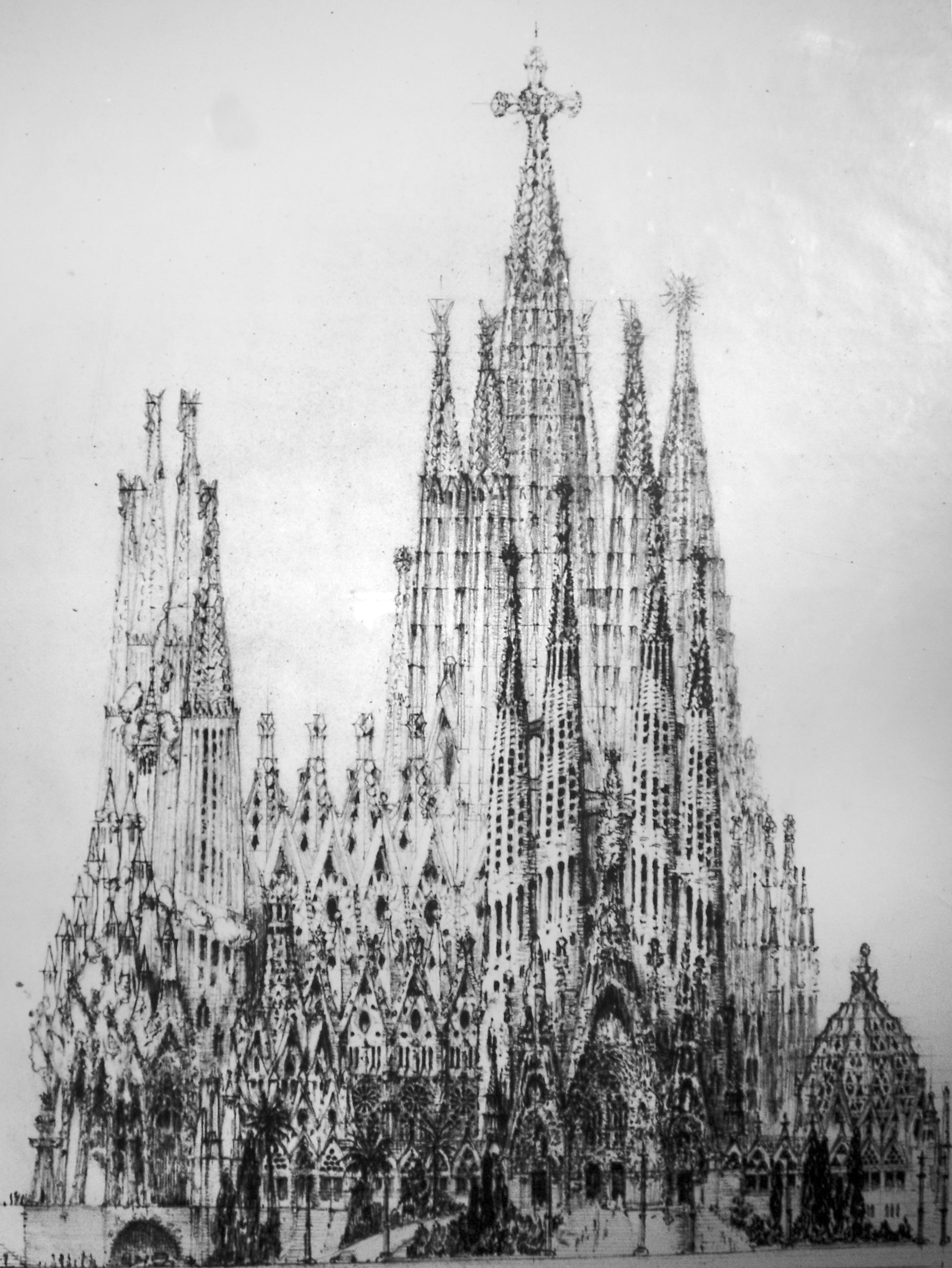
Figure 27: Lluís Bonet i Garí’s interpretation (circa 1945) of what the Sagrada Família would look like when completed. The tall central tower capped by a cross is dedicated to Jesus Christ.
High above the main crossing of Basílica de la Sagrada Família, Antoni Gaudí planned a tall central tower dedicated to Jesus Christ (fig. 27). The tower marks the basilica’s apex of 170 metres and the culmination of a design that has been in development for over one hundred years. Today, almost eighty-five years after Gaudí’s death in 1926, the team of architects continuing his work is preparing to construct the central tower.
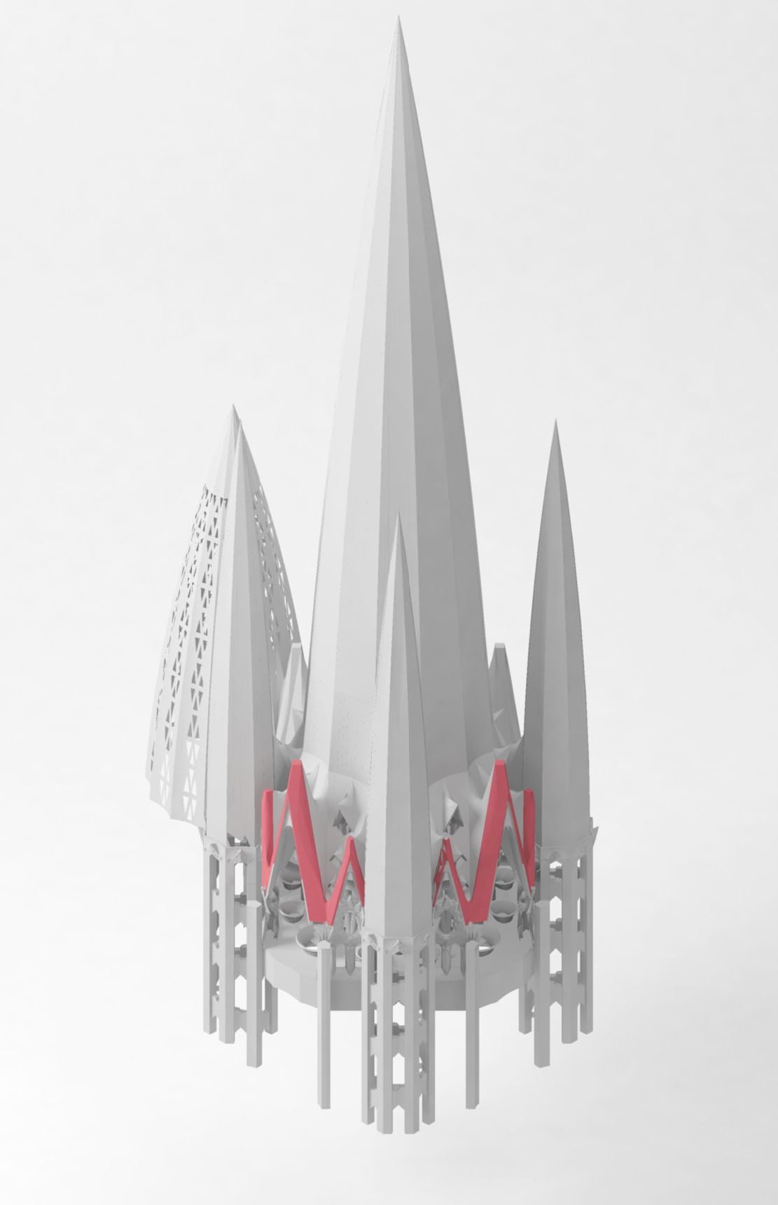
Figure 28: A massing model of the central tower with the frontons highlighted in red.
At the base of the tower sit three matching gabled windows, each seventeen metres high (fig. 28). The stone head to these windows is called a fronton by the project team (fronton being Catalan for gable). The fronton design, like everything else on the church, has stretched over a period of years. The progression of software in this time has seen the digital fronton model pass from one CAD version to the next. At some stage during this process, the parametric relationships in the fronton model were removed and the model became explicit geometry. In 2010, as the project team were preparing the fronton’s construction documentation, they came across a curious problem with the model: passing the model between software had caused slight distortions. With the parametric relationships removed, fronton faces that should have been planar contained faint curves, lines that should have been orthogonal were a couple of degrees off, and geometry that should have been proportional was just a touch inconsistent (fig. 29 & 30). None of these distortions were apparent at first glance and on a more routine project they probably would not be of concern. However, on a project as meticulous as the Sagrada Família – where the design has germinated for decades – it was vitally important to remove any imperfections, or at least get them within the tight tolerances of the seven-axis robot scheduled to mill the stone. My task was to straighten the explicit geometry in the fronton model by converting it back into a parametric model and reasserting the original parametric relationships.
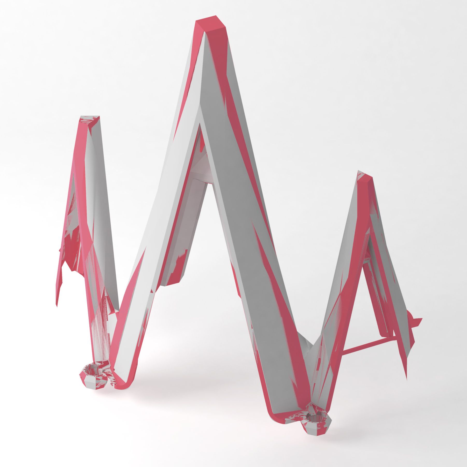
Figure 29: The original fronton model (red) overlaid with the corrected model (grey). The slight distortions in the original model cause some parts to disappear behind the corrected model while other parts push out and envelop the corrected model.
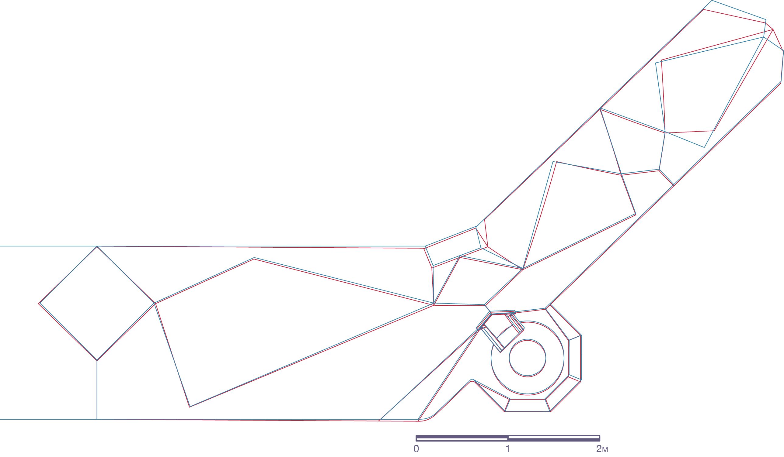
Figure 30: Blue: Plan of original fronton model. Red: Plan of corrected model. The two plans deviate 6mm on average.
The realignment of the frontons presents a unique parametric modelling case study. Besides contributing to one of the earliest examples of parametric architecture, the project demands an extraordinary level of precision, while the ambiguity of what constitutes straightened requires collaboration with team members in Melbourne and Barcelona. This case study is not necessarily representative of typical parametric architecture projects but, as I discussed in chapter 4.1, the project’s unique circumstances offer what Robert Stake (2005, 451) calls “the opportunity to learn.” In this chapter I observe how the demands of the fronton realignment manifest within two parametric models. In particular, I examine how the language paradigm of the parametric model affects its behaviour (following on from chapter 3.2, where I noted most parametric models are based on a narrow range of language paradigms). I begin this chapter by discussing the taxonomy of possible language paradigms and identifying how the rarely used logic programming paradigm may be applicable to parametric modelling. I then twice realign the frontons, once with a conventional dataflow parametric model, and once with a parametric model based on logic programming. The differences between these two language paradigms form the discussion of this chapter.
5.2 – Programming Paradigms
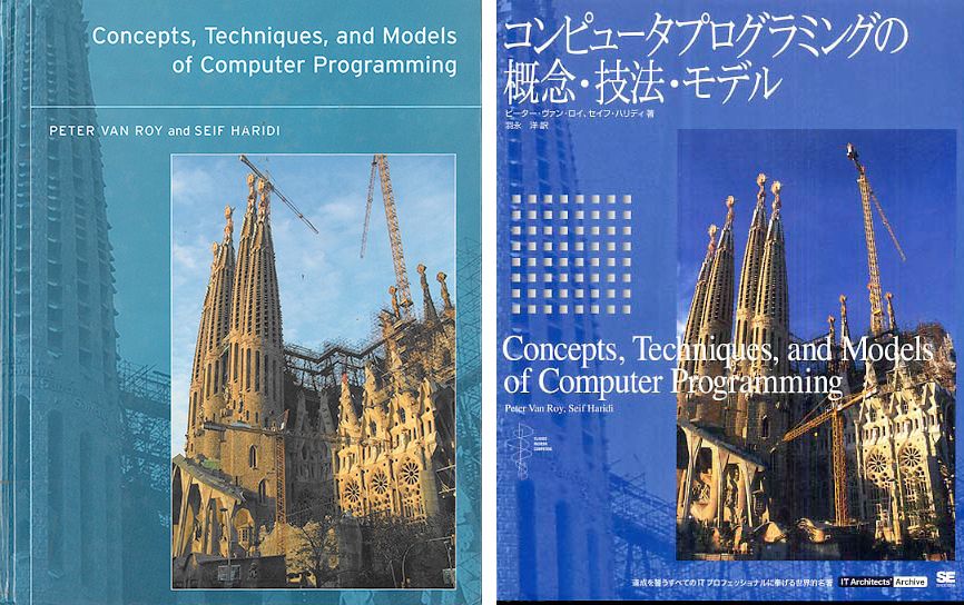
Figure 31: Van Roy’s photograph of the Sagrada Família on the cover of Concepts, Techniques, and Models of Computer Programming (Van Roy and Haridi’s 2004). The Japanese edition uses a slightly different photograph of the Sagrada Família.
The Sagrada Família graces the cover (fig. 31) of Peter Van Roy and Seif Haridi’s (2004) seminal book on programming languages entitled Concepts, Techniques, and Models of Computer Programming. Van Roy took the photograph and chose it for the cover because “the still unfinished Expiatory Temple of the Sagrada Família in Barcelona is a metaphor for programming” (Van Roy, n.d.). Van Roy and Haridi never foresaw, however, that the opposite maybe true, that the programming paradigms they discuss in their book could help designers of the church on its cover. In the preface Van Roy and Haridi (2004, xx) allude to another architect, Mies van der Rohe, in a section about programming paradigms titled “more is not better (or worse), just different.” A programming paradigm in this context is the set of underlying principles that shape the style of a programming language. For Van Roy and Haridi, these styles are not better nor worse, just different to one another. It is this difference that I consider in relation to the parametric models of the Sagrada Família.
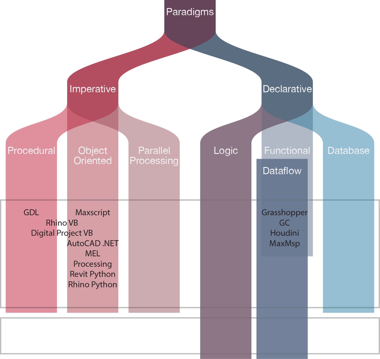
Figure 32: The programming languages architects use categorised by Appleby and VandeKopple’s (1997, xiv) taxonomy of programming paradigms. The two paradigms explored in this case study are logic programming and dataflow programming.
Programming paradigms are roughly divided by Van Roy and Haridi (2004) as well as others like Appleby and VandeKopple (1997) into imperative paradigms or declarative paradigms (fig. 32). Imperative languages describe a sequence of actions for the computer to perform – much like imperative verbs in the English language. In contrast, declarative languages “define the what (the results we want to achieve) without explaining the how (the algorithms needed to achieve the results)” (Van Roy and Haridi 2004, 114). Imperative and declarative languages can be further classified into more specific paradigmatic subcategories, as shown in figure 32. Most programming languages are based on at least one of these subcategories, and many spread out to embody multiple paradigms within the one language – more is not better (or worse).
As discussed in chapter 3.2, the languages favoured by designers tend to occupy a narrow range of possible paradigms (fig. 32). The major textual CAD programming languages are all predominantly imperative1 with a bias towards procedural imperativeness. This is not surprising considering that the world’s five most popular programming languages on the TIOBE (2012) index are also predominantly imperative2 (although perhaps more spread out on the imperative spectrum). In contrast, visual programming languages tend towards declarativeness. The major visual CAD programming languages all reside in a very narrow subsection of declarative programming known as dataflow programming.3 In this chapter I compare two declarative paradigms – dataflow programming and logic programming – as a means to construct the parametric models of the Sagrada Família frontons.
5.3 – Challenges of Dataflow
In the introduction to Data Flow Computing, John Sharp (1992, 3) defines a dataflow program as “one in which the ordering of operations is not specified by the programmer, but that is implied by the data interdependencies.” In other words, a dataflow language describes the connections between computational operations, which is different to the imperative approach of listing operations in the order they should occur. When a dataflow program is run, the computer infers the precise order of operations from the stated connections between operations.

Figure 33: The parts of a DAG.
The quintessential example of a dataflow program is a spreadsheet. The user of a spreadsheet specifies how cells connect and how cells should process data but leaves the computer to decide the precise order in which cells get updated. The same principle applies to certain parametric modelling software, like Digital Project. Users of this software specify a network of connections between geometric operations while the computer manages the exact sequencing and execution of these operations. Many visual programming languages operate on a similar principle since the connections between operations can be represented using a type of flow-chart know as a Directed Acyclic Graph (DAG). The two components of a DAG are nodes and directed edges (fig. 33). In a visual program a node represents an operation and a directed edge represents a connection (a flow of data between two operations), which is how the visual programming environments used by architects (Grasshopper, GenerativeComponents, and Houdini) represent dataflow programs.4
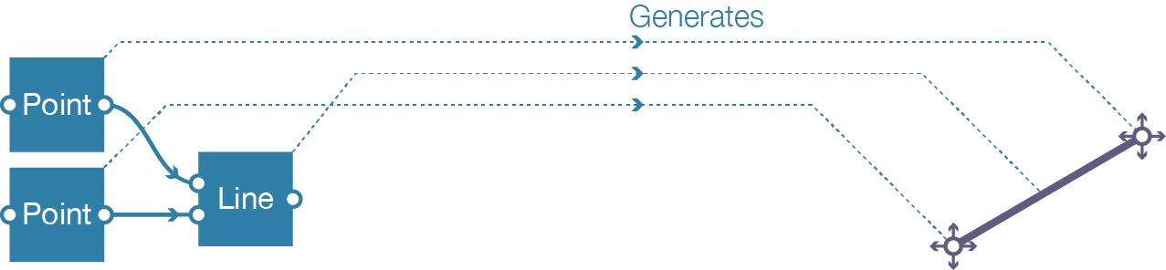
Figure 34: The relationship between a DAG and the geometry it generates. In the DAG the line is a child of the two points, accordingly, the line’s geometry depends entirely on the location of the points. Moving the geometry of either point would also move the line.
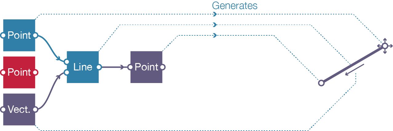
Figure 35: Modifications to the DAG from figure 34. The geometry is the same but the connections have been changed: one of the points is now a child of the line. In the geometric model, the child point can no longer be moved directly since its location now depends on the line’s position (the parent of the point). While the geometry is the same as figure 34, the change in hierarchy requires adding and removing a number of nodes. Blue: Existing nodes. Purple: New nodes. Red: Deleted nodes (from figure 34).
5.4 – Logic Programming
Logic programming, like dataflow programming, fits into the declarative branch of programming paradigms (fig. 32). Defined by Sterling and Shapiro (1994, 9), the first part of “a logic program is a set of axioms, or rules, defining relations between objects.” These relations do not specify flows of data but rather express, in first order logic, statements of fact. For example, an axiom might be: A cat is an animal. The second part of a logic program is an interpreter that reads the axioms and logically deduces the consequences (Sterling and Shapiro 1994, 9).5 Using the above axiom, the interpreter might be asked what is an animal? to which it would deduce: cat.
At the genesis of logic programming, in the late 1960s and early 1970s, many expected logic programming’s formalisation of human reasoning to push humanity beyond its cognitive limitations (limitations that had ostensibly brought about events like software crisis). Robert Kowalski (1998) recalls his contemporaries during this period employing logic programming for ambitiously titled projects involving “natural language question-answering” (38) and “automated theorem proving” (39). The initial developments were promising with researchers discovering various ways to get computers to seemingly reason and respond to a series of questions, even if the questions were always confined to small problem domains (Hewitt 2009). The hope was that if a computer could answer a simple question like how many pyramids are in the blue box? then it would be possible to get a computer to answer a more difficult question like What does “cuantas pyramides se encuentran dentro de la caja azul” mean? But, as I have discussed in chapter 3, systems addressing small problems – be they computer programs or parametric models – do not always scale to address larger problems. The initial interest in logic programming waned as success with small, well-defined problems failed to bring about widespread success with larger problems. Today the most common logic programming language – Prolog – only ranks thirty-sixth on the TIOBE (2012) index of popular programming languages. Nevertheless, logic programming still finds niche applications in expert reasoning – particularly expert reasoning about relationships (for instance, IBM’s Jeopardy winning computer, Watson, was partly based on Prolog [Lally and Fodor 2011]).
In the architecture industry, logic programming followed a similar arc, albeit a few years behind what was happening in software engineering. Architectural researchers took the work done on spatial logic programming and enthusiastically applied it to a favourite problem of the time: room layout (Keller 2006). A paper typical of the period is Peter Swinsons’ (1982) optimistically named Logic Programming: A Computing Tool for the Architect of the Future. In this paper Swinson (1982, 104) demonstrates how Prolog can solve four different layout problems before concluding “this new way of programming does indeed hold much promise for the future” (a similar method is used by Márkusz [1982]). A flurry of interest followed in the 1980s.6 In 1984, Gonzalez et al. demonstrated two-dimensional drafting using logic programming, which they found “more concise, more reliable, and clearer” as well as “more efficient” than imperative programming (Gonzalez et al. 1984, 74). Further examples of two-dimensional shape drawing were given by Brüderlin (1985) and subsequently Helm and Marriott (1986). A more comprehensive attempt to generate three-dimensional models was made by Robert Woodbury (1990) using the ASCEND language, which is not strictly a logic programming language although it shares many similarities. The zenith for logic programming in architecture was arguably reached the same year with the publication of William Mitchell’s (1990) The Logic of Architecture.
Despite The Logic of Architecture’s success, it marks the beginning of the end. While Mitchell was able to apply his ideas retrospectively to Palladian villas, he never tested them on real architecture projects. Indeed, none of the papers I have referenced (or that I can find) discuss using logic programming on real architecture projects – even though many of them, like Swinson, were making confident proclamations that logic programming would become the “computing tool for the architect of the future” (Swinson 1982). Much like the software engineers that came before them, these researchers all tested logic programming with small, idealised problems assuming the success of these small systems were representative of future successes at larger scales. The initial interest in logic programming waned (like it had done in software engineering a few years earlier) as success with small, well-defined problems failed to bring about widespread success with larger problems. Nevertheless, there are still a couple of recent examples of logic programming being used by researchers (still on small, idealised problems) including Martin and Martin’s PolyFormes tool (1999) and Makris et al. MultiCAD (2006). However, in contrast to the widespread imperative programming paradigm used by architects, logic programming never quite became the computing tool for the architect of the future. In fact, I can find no example of logic programming ever being used on a real architecture project.
The following case study differs from prior logic programming research in three important ways. Firstly, it investigates logic programming in the context of a real design problem from the Sagrada Família rather than discussing logic programming theoretically applied to an idealised problem. Secondly, it focuses on deducing the hierarchy of relationships for a parametric model instead of directly generating geometry, or laying out rooms, or drawing Palladian villas. Finally, this research does not aspire to develop the computing tool for the architect of the future; instead it aims to observe how programming paradigms influence the flexibility of parametric models.
5.5 – Logic Programming Parametric Relations
As part of my research I developed a logic programming language for generating parametric models. A designer using the language can specify connections between operations, which are then used by an interpreter to derive the flow of data without the designer needing to specify a hierarchy (like they would in a dataflow language). I elected to develop my own logic programming interpreter in C# rather than using an existing logic programming implementation. This allowed me to link the interpreter directly to a parametric engine I had already built on-top of Rhino 4’s geometric API (an engine reused for the case study in chapter 7).
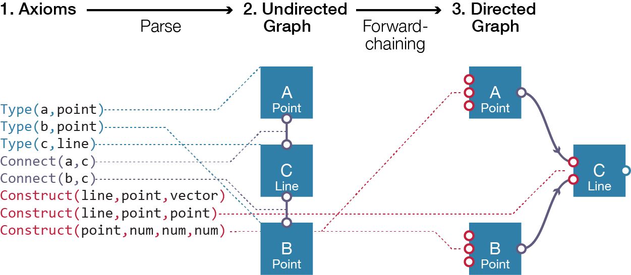
Figure 36: The major stages involving in deducing a parametric model to satisfy a set of textual axioms. The dashed lines show how the axioms generate particular parts of the graphs in the various stages.
My logic programming interpreter uses a three-stage process to derive a parametric model automatically from a set of axioms. These stages are illustrated in figure 36. The first stage is to read the text file containing the axioms. In the second stage, the axioms are parsed into an undirected graph (using rules I will explain shortly). At the final stage, the interpreter uses forward-chaining to deduce the directness of the graph, which produces the DAG of a parametric model satisfying the initial axioms.
There are three types of axioms permitted in the language:
Axiom Type 1: Geometric
A geometric axiom defines a geometric entity’s unique name and geometry type. For example, a line with the name of C, is defined by the axiom: type(C,line).
Axiom Type 2: Connection
A connection axiom establishes a connection between two geometric entities. For example, to connect line C to point B, the axiom would be: connect(B,C). Connection axioms do not define the direction of the connection, they only state that two geometric entities are related.
Axiom Type 3: Construction
A construction axiom describes a combination of parents that define a particular geometry type. For example, a line can be defined by two parent points, which is expressed with the axiom: construct(line,point,point). Any particular geometry type can have multiple construction axioms. For example, a line may also be defined by a point and a vector: construct(line,point,vector). Using forward-chaining, the interpreter selects the most appropriate construction axiom for a given situation. In figure 36, the forward-chaining algorithm has inferred that node C, a type of line, must be defined by two parent points. To satisfy this relationship, the interpreter organises the undirected graph into a hierarchy so that line C becomes the child of the two points (A & B). The following page explains the three rules used to infer the most appropriate construction axioms.
Inference 1: Asymmetric constructors
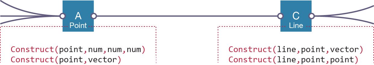
Figure 37: A must be the parent of C, since none of the construction axioms for A require a line as a parent, whereas both the construction axioms of C require a point as a parent.
The construction axioms list the type of geometry that can act as the parent for any given type of node. If two nodes are connected, and the first node has a construction axiom allowing the second node to be its parent, and the second node does not have any construction axioms that allow the first node to be its parent, then the first node must necessarily be the parent of the second node.
Inference 2: Constructor elimination
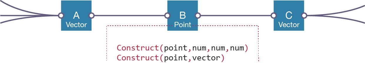
Figure 38: The first construction axiom requires B to have three parents that are numbers. Since B is not connected to any numbers, it will never be able to fulfil this axiom and therefore the axiom can be eliminated. The second axiom is still possible, which means one of the vectors much be a parent to B.
If a node has multiple construction axioms, some axioms can be eliminated if the node is not connected to the right combination of node types to fulfil a particular construction axiom. Eliminating constructor axioms makes it more likely to find asymmetric constructors.
Inference 3: Constructor definition
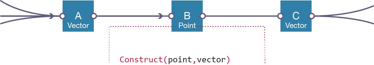
Figure 39: If A is B’s parent, then B’s construction axiom is fulfilled and it cannot have anymore parents. Accordingly, all the remaining undirected connections must flow away from B, and thus C is a child of B.
If a node has all the required parents to fulfil a construction axiom, then it does not need any more parents and all the remaining nodes connected through undirected connections must be children. Once this rule becomes relevant the directedness normally cascades through the graph as large numbers of connections become directed.
Ideally these three rules are enough to deduce the entire flow of the graph. On occasion the axioms will define an over-constrained graph, producing a situation where two nodes are connected but neither is a permissible parent of the other. In this case the interpreter first looks to see if the addition of numerical nodes will allow progress past this impasse. If not, the user is asked to resolve the axiom conflicts.
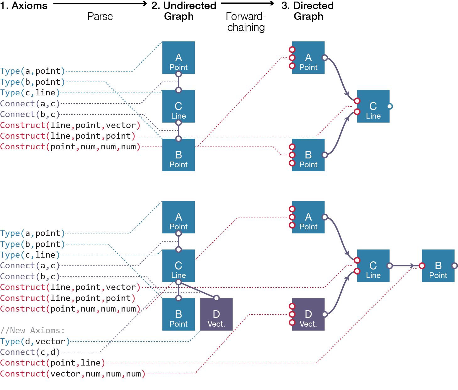
Figure 40: An example of how changes to a set of axioms translate into changes within a parametric model. Top: The axioms and resulting parametric model from figure 36. Bottom: The inclusion of new axioms creates a slightly different undirected graph which the forward-chaining interpreter transforms into a radically different parametric model when compared to the one above (note that these changes are the same as with the dataflow model in figure 35).
A designer using this logic programming system only needs to define connections between geometric entities, which leaves the interpreter to infer the direction of the connections. Figure 40 shows how axioms transform into a parametric model and how changes to the axioms automatically result in new dataflows. The example in figure 40 is identical to the earlier dataflow example in figure 35 except, unlike the dataflow example, the changes to the parametric model’s hierarchy are managed invisibly by the interpreter; the designer adds a few axioms and the new dataflow is automatically derived by the interpreter. The following section describes how these changes come to impact real architecture projects.
5.6 – Application to the Sagrada Família
Every vertex was slightly awry on the Sagrada Família’s fronton model. This introduced curves to faces that should have been planar, pulled geometry out of line with important axes, and unsettled the proportions of the model (fig. 29). In March 2010, I developed a set of parametric models to realign the vertices of the distorted model. I built these models from Melbourne, Australia and was guided by discussions with Mark Burry and the Sagrada Família design office based in Barcelona, Spain.
To understand the impact of a parametric model’s programming paradigm, I straightened the frontons twice: once with a dataflow language, and once with a logic programming language. In order to do so, the geometry of the frontons was first converted into a parametric model in each of the respective programming paradigms. Once converted, parametric relationships were introduced to realign the model. These relations ensured that polygons were regular and that certain groups of vertices were planar, symmetrical, proportioned, and on an axis. The parametric model was then flexed so the new geometry matched the original model as closely as possible.7 The specific process of using dataflow programming and logic programming was as follows.

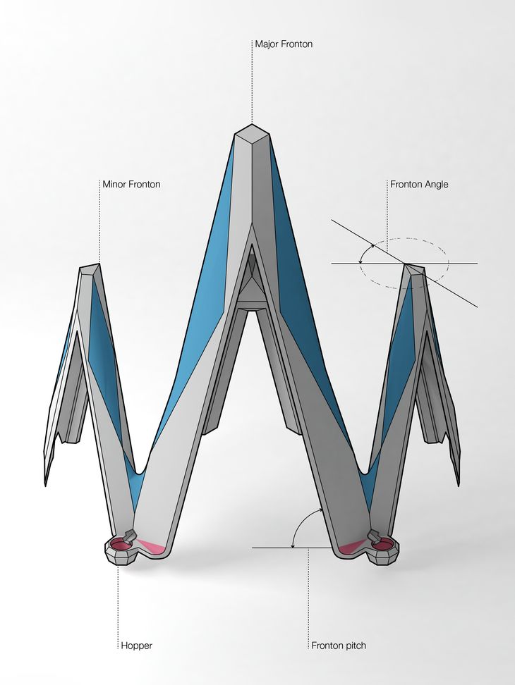
Figure 41: The key parts of the Sagrada Família’s frontons. Like much of Gaudí’s architecture, the frontons consist of ruled surfaces: Grey: Planar surfaces. Blue: Hyperbolic paraboloids. Red: Conic sections.
Applying Dataflow
The dataflow parametric model contained approximately a thousand geometric operations that straightened the one hundred and eleven vertices in the original fronton model. This parametric model was as large as the largest models analysed in chapter 4.3.8 Due to the anticipated size of the model, I elected to generate the fronton parametric model in Digital Project. The geometry was imported into Digital Project where I introduced parametric relationships to fix the original model’s distortions. The parameters of the Digital Project model were managed in an Excel spreadsheet. By changing values in the spreadsheet I could move the new refined frontons as close as possible to the original geometry. The best set of parameters I could find reduced the median difference between the two models to 13mm. I then further refined these values using a genetic algorithm, which narrowed the median distance to 6mm. Since it was only the model’s parameters being changed, all the parametric relationships in the new geometry were maintained during this process.
Applying Logic Programming
The frontons were also straightened with the logic programming technique I described earlier. The logic programming environment took a series of axioms describing the frontons’ geometric relationships and then derived a parametric model to satisfy these relationships. In total, approximately six hundred axioms were required to generate the parametric model of the frontons. Almost five hundred axioms were automatically generated. These included most of the geometric axioms, which could be found by iterating through all the points, lines, and planes in the original model to produce axioms like: type(p_127,point) and type(plane_3,plane). Most of the connection axioms were found using a similar method whereby vertices from lines or planes that coincided with a point were said to be connected, which produced axioms like: connect(p_127,plane_3). The remaining one hundred axioms in the logic programming model were generated manually. These included the construction axioms, as well as new geometric axioms to define important planes, axes, polygons, and vectors. From these axioms the logic programming interpreter generated a parametric model. The model’s parameters were refined using a genetic algorithm, which reduced the median distance between the new and old model to 6mm – a comparable result to the dataflow model.9
5.7 – Analysis of Programming Paradigms
Method
Straightening the Sagrada Família’s frontons with a logic programming paradigm and a dataflow paradigm presents the opportunity to observe how the programming paradigms affect the respective parametric models. The following observations draw upon the research instruments discussed in chapter 4. Of particular interest is how the programming paradigm impacts the model’s construction time as well as the relative modification time and extendability. In addition, the latency between changes and the verification of model correctness are important differentiators between the two paradigms.
Construction Time
Constructing the first version of the dataflow parametric model in Digital Project and Excel took approximately twenty-three hours. This time does not include the time taken to convert the original geometry into Digital Project or the subsequent time spent modifying the first version of the parametric model. Much of the twenty-three hours was consumed selecting the appropriate parametric relationships, working out how to apply the relationships in a hierarchy of parent-child connections, and verifying the relationships generated the expected geometry. Working out the correct parent-child connections was deceptively difficult since connections often had flow-on implications for the surrounding geometry. These challenges were largely avoided with logic programming by generating the majority of the axioms automatically from the existing geometry and by using the logic programming interpreter to infer the hierarchy of relationships these connections imply. Accordingly, constructing the first version of the logic programming parametric model took approximately five hours.
In this case using a logic programming paradigm was four to five times faster than using a dataflow paradigm. The time difference is largely attributable to the automatic extraction of axioms and subsequent inference of the model’s hierarchy with the logic programming interpreter. This was only possible because there was a pre-existing geometric model of the frontons, which is an unusual circumstance for most architecture projects. The difference in construction time cannot therefore be expected on other architecture projects, particularly ones without a pre-existing geometric model. Nevertheless, the variance in construction time demonstrates that programming paradigms can significantly affect projects, although these affects are dependent upon the circumstances of the project. An appropriate circumstance for logic programming seems to be when a pre-existing explicit geometric model needs to be converted into a parametric model.
Modification Time and Extendability
Modification time is a quantitative measure of how long a change takes to make while extendability is a qualitative assessment of the ease with which a program adapts to change (Meyer 1997, 6-7). In straightening the frontons there were two primary changes asked for, both of which reinforce the precision required in the project:
- Minor Fronton Angle: On the original distorted model the minor fronton axis angle was 43.875 degrees (fig. 41). I initially ‘corrected’ this to 45.000 degrees, which caused the model to move significantly. The design team asked the angle be changed back to 43.875 degrees before subsequently deciding that 43.904 degrees was most in keeping with the geometry of the Sagrada Família’s central tower. When I built the dataflow model I was uncertain of the fronton angle so I included a parameter to control it. This parameter permitted these changes to be made almost instantaneously. On the logic programming model the changes could be accommodated by adding a new axiom to define the vector of the plane linked to the centre of the minor fronton. This process took slightly longer than in the dataflow language, but still less than fifteen minutes.
- Minor Fronton Pitch: In one of the final iterations it was discovered that the pitch of the major and minor frontons was slightly different. I had come across the anomaly previously but assumed it was a rounding error since the deviation was less than 0.02 degrees. Over a ten metre span this slight abnormality resulted in a 2mm error, which was outside the tolerance of the seven-axis robot milling the frontons. The solution was to redefine the pitch of the minor fronton. In the dataflow model this change had few flow-on consequences and therefore took less than thirty minutes to implement. The logic programming language unfortunately lacked the vocabulary to express the pitch change. I spent two hours adding a new construction axiom to the logic programming vocabulary that permitted a vector to be mirrored through a plane. Once this axiom was added, it took approximately fifteen minutes to change the pitch of the minor fronton by mirroring the pitch of the major fronton.
On this project both programming paradigms were extendable enough to accommodate both of the primary changes. The changes were somewhat unusual in that they did not affect the topology of the project (an act many authors I discussed in chapter 2.3 found disruptive). The changes instead focused on the precision of the model and the way the geometry was related. In making these changes the dataflow language offered slightly faster modification times: in the first case because I anticipated the change by including a parameter for it, and in the second case because logic programming was slowed by limitations in its vocabulary. This success does not confirm the agility of dataflow programming as much as it confirms the importance of the designer’s intuition in setting up a model’s hierarchy, and the importance of what Meyer (1997, 12-13) calls the modelling environment’s functionality (having the right vocabulary to express an idea or change).
In retrospect the changes to the frontons seem relatively minor for the effort expended on them. However, the magnitude of these changes comes from the model extendability rather than the brief. Had I been using a non-parametric model, or had I created an inflexible parametric model, both of these changes would have involved deleting over half of the model’s geometry and starting again. The minor changes would have been serious problems. Thus, while the attention to detail on the Sagrada Família may seem pedantic, the level of design consideration is only afforded by maintaining flexible representations.
Latency
Latency measures the delay in seeing the geometry change after changing a model’s parameters. With the dataflow model, modifications to the Excel values would propagate out into the geometry produced by Digital Project within a few seconds, which was not quite real-time but near enough for this project. Conversely, the logic programming model had a pronounced latency between editing the axioms and seeing the resulting geometry. Minutes would elapse while the interpreter worked to derive the parametric model after axiom changes.10 Since the derived parametric model did not always have parameters in intuitive places, often the only way to change numerical values (like the angle of the minor fronton) was to change the axioms and then wait as the interpreter derived a new parametric model. This latency made changing the logic programming model a more involved and less intuitive process than with the dataflow model.
Correctness
Correctness describes whether a program does what is expected (Meyer 1997, 4-5). For both programming paradigms it was difficult to verify the models were doing what was expected. In the dataflow language the quantity of relationships obfuscated the flow of data, which made it hard to work out what the model should have been doing. On three occasions this led to the wrong geometric operation being applied. These errors were not apparent by looking at the dataflow model or by visually inspecting the geometry, and they were only caught by the project architects manually measuring the model. Logic programming was equally difficult to verify because it was not always apparent how the geometry derived from the axioms. Often I would end up adding axioms one-by-one to understand their impact on the final geometry. In the end, both programming paradigms produced parametric models that did what was expected but, in a project where the geometric changes were subtle and the relationships numerous, often the only way to verify correctness was to examine what the model did rather than understand how the model did it.
5.8 – Conclusion
Van Roy and Haridi (2004, xx) write that when it comes to programming paradigms “more is not better (or worse), just different.” Yet for architects applying parametric models to projects like the Sagrada Família, they have always had less than more when it comes to programming paradigms. Architects building parametric models are presently confined to either declarative dataflow paradigms in visual programming languages, or procedural imperative paradigms in textual programming languages. The research I have presented demonstrates that programming paradigms influence – at the very least – the parametric model’s construction time, modification time, latency, and extendability. Since programming paradigms cannot normally be switched without rebuilding a model, selecting an appropriate programming paradigm for the context of a project is a critical initial decision. This is a decision that has an evident affect on many aspects of a parametric model’s flexibility yet, unfortunately, it is a decision largely unavailable to architects; they often cannot choose more, less, or different – just: dataflow or procedural. Van Roy and Haridi’s discussions of programming languages are interesting, not just because Van Roy sees the Sagrada Família as a metaphorical signifier of them, but because these discussions of programming paradigms signify how parametric models, like those used on the Sagrada Família, can be tuned to privilege different types of design changes.
Perhaps the most intriguing part of this case study is the disjunction between the theoretical advantages of logic programming and the realised advantages of logic programming. I began this chapter by talking about the challenges of modifying the hierarchy of relationships in a dataflow language and I postulated that the time associated with these modifications could theoretically be reduced if the computer – rather than the designer – organised the parametric model’s hierarchy. In a series of diagrams I illustrated how a logic programming language would allow a designer to specify directionless connections that are automatically organised by a logic programming interpreter, thereby reducing the theoretical modification time. Yet in reality the opposite happened: when used to generate the parametric model of the Sagrada Família’s frontons, logic programming actually lengthened the modification time. This is in large part because the interpreter often took a long time to generate a new instance of the model – a detail easily overlooked when discussing logic programming theoretically, but one that can possess significant importance when a designer has to wait five minutes for the logic programming interpreter to work through the six hundred axioms in order to realise a single modification to the frontons. While these results are highly dependent upon circumstance – and although the Sagrada Família’s size, detail, and precision makes it a rare circumstance – these results do underscore the value of practice-based understandings of parametric modelling. This disjunction between theory and practice when talking about programming paradigms is perhaps the reason why logic programming failed to live up to the theoretical expectations that had been expressed by authors who had never actually used logic programming in practice – examples include, Mitchell (1990) in The Logic of Architecture and Swinson (1982) in Logic Programming: A computing tool for the architect of the future.
While logic programming did not live up to Mitchell or Swinson’s hopes, and while logic programming induced a far greater latency than I expected in theory, this is not to say logic programming is without merit. Logic programming in architecture, as in software engineering, appears to excel at reasoning about relationships. In this capacity, it seems particularly suited to extracting relationships from pre-existing geometry in order to derive a parametric model; the reverse of the typical parametric modelling process. In the fronton case study, with a pre-existing geometric model of the frontons, this led to significantly reduced construction times when compared to the dataflow model. However, both methods produced large and intricate models that were hard to verify as being correct – an issue of understandability addressed in the following chapter.
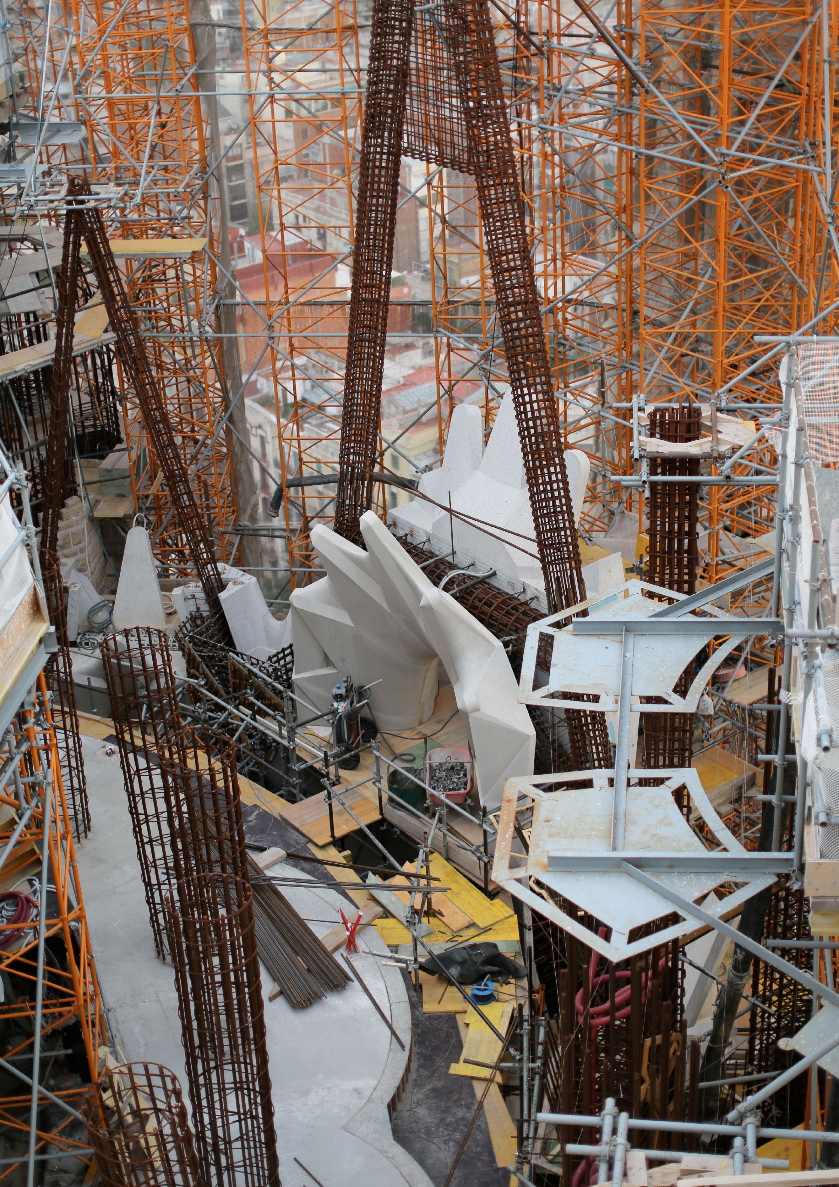
Figure 42: The frontons under construction at The Sagrada Família in September 2012.
Thesis Navigation
- Return to table of contents
- Goto previous chapter
- Goto next chapter
- Download entire thesis as PDF (30mb)
Footnotes
1:These include: 3dsMax: Maxscript; Archicad: GDL; Digital Project: Visual Basic; Maya: Maya Embedded Language; Processing: Java; Revit: Visual Basic & Python; Rhino: Visual Basic & Python; Sketchup: Ruby.
2:As of May 2012 the worlds five most popular programming languages, as measured by TIOBE (2012), are: C, Java, C++, Objective-C, and C#.
3:These include: Grasshopper; GenerativeComponents; Houdini; and MaxMsp.
4:I discuss, in chapter 7, an alternative way to represent a dataflow program textually rather than visually.
5:On the surface, there may appear to be many examples of logic programming used in CAD. For example, Sketchpad (Sutherland 1963), has a geometric constraint solver that allows users to define axioms between geometry. However, Sketchpad does not satisfy the definition of logic programming since the axioms are interpreted using numeric algorithms and an early form of hill climbing rather than through logical deduction (Sutherland 1963, 115-19). The logical deduction that forms the basis for logic programming was not invented until six years after Sketchpad.
6:For a complete history see: Fudos 1995.
7:Closeness in this case was measured as both the median distance model vertices moved and the maximum distance model vertices moved.
8:Figure 27 & 28 show how the fronton model is only a small component of the Sagrada Família overall, and a fairly geometrically simple component at that. To have such a large and detailed architecture project modelled parametrically is quite unusual. And with parametric models being employed on the Sagrada Família for almost two decades, I would venture to say that in aggregate the models are likely to be the most extensive and most complex parametric models ever used in an architecture project.
9:The genetic algorithm initially proved ineffective on the parametric models produced by logic programming since the logic programming interpreter initialised all values to zero, which caused the optimisation to begin thousands of millimetres from its target. In pulling the geometry towards the target, the genetic algorithm had a tendency to get stuck on local optima. To overcome this problem, the values of the model were initialised using a hill climbing algorithm. This got the geometry into approximately the right place before the final refinement with the genetic algorithm.
10:The latency increases with model size although it may be influenced by other factors. These include the interpreter’s efficiency and the way the axioms define the problem. The results discussed should not be interpreted as evidence that logic programming suffers from general latency issues, rather the results should be read with the caveat that they are particular to the project’s specific logic programming implementation and to the specific circumstances of this project.
Bibliography
Appleby, Doris, and Julius VandeKopple. 1997. Programming Languages: Paradigm and Practice. Second edition. Massachusetts: McGraw-Hill.
Brüderlin, Beat. 1985. “Using Prolog for Constructing Geometric Objects Defined by Constraints.” In Proceedings of the European Conference on Computer Algebra, edited by Bob Caviness, 448-459. Linz: Springer.
Davis, Daniel, Jane Burry, and Mark Burry. 2011c. “The Flexibility of Logic Programming.” In Circuit Bending, Breaking and Mending: Proceedings of the 16th International Conference on Computer Aided Architectural Design Research in Asia, edited by Christiane Herr, Ning Gu, Stanislav Roudavski, and Marc Schnabel, 29–38. Newcastle, Australia: The University of Newcastle.
Fudos, Ioannis. 1995. “Constraint Solving for Computer Aided Design.” PhD dissertation, Purdue University.
Gonzalez, Camacho, M. Williams, and E. Aitchison. 1984. “Evaluation of the Effectiveness of Prolog for a CAD Application.” IEEE Computer Graphics and Applications 4 (3): 67-75.
Helm, Richard, and Kim Marriott. 1986. “Declarative Graphics.” In Proceedings of the Third International Conference on Logic Programming, 513-527. London: Springer.
Hewitt, Carl. 2009. “Middle History of Logic Programming: Resolution, Planner, Edinburgh LCF, Prolog, Simula, and the Japanese Fifth Generation Project.” arXiv preprint arXiv:0904.3036.
Keller, Sean. 2006. “Fenland Tech: Architectural Science in Postwar Cambridge.” Grey Room 23 (April): 40-65.
Kowalski, Robert. 1988. “The Early Years of Logic Programming.” Communications of the Association for Computing Machinery 31 (1): 38-43.
Lally, Adam, and Paul Fodor. 2011. “Natural Language Processing With Prolog in the IBM Watson System.” The Association for Logic Programming (ALP) Newsletter. Published 31 March. http://www.cs.nmsu.edu/ALP/2011/03/natural-language-processing-with-prolog-in-the-ibm-watson-system/.
Makris, Dimitrios, Ioannis Havoutis, Georges Miaoulis, and Dimitri Plemenos. 2006. “MultiCAD: MOGA A System for Conceptual Style Design of Buildings.” In Proceedings of the 9th 3IA International Conference on Computer Graphics and Artificial Intelligence, edited by Dimitri Plemenos, 73-84.
Martin, Philippe, and Dominique Martin. 1999. “PolyFormes: Software for the Declarative Modelling of Polyhedra.” The Visual Computer 15 (2): 55-76.
Mitchell, William. 1990. The Logic of Architecture: Design, Computation, and Cognition. Massachusetts: MIT Press.
Márkusz, Zsuzsanna. 1982. “Design in Logic.” Computer-Aided Design 14 (6): 335-343.
Meyer, Bertrand. 1997. Object-Oriented Software Construction. Second edition. Upper Saddle River: Prentice Hall.
Sharp, John. 1992. “A Brief Introduction to Data Flow.” In Dataflow Computing: Theory and Practice, edited by John Sharp. Norwood: Ablex.
Stake, Robert. 2005. “Qualitative Case Studies.” In The SAGE Handbook of Qualitative Research, edited Norman Denzin and Yvonnas Lincoln, 443-466. Third edition. Thousand Oaks: Sage.
Sterling, Leon, and Ehud Shapiro. 1994. The Art of Prolog: Advanced Programming Techniques. Second edition. Massachusetts: MIT Press.
Swinson, Peter. 1982. “Logic Programming: A Computing Tool for the Architect of the Future.” Computer-Aided Design 14 (2): 97-104.
TIOBE Software. 2012. “TIOBE Programming Community Index for May 2012.” Published May. http://www.tiobe.com/index.php/content/paperinfo/tpci/index.html.
Van Roy, Peter, and Seif Haridi. 2004. Concepts, Techniques, and Models of Computer Programming. Massachusetts: MIT Press.
Van Roy, Peter. n.d. “Book Cover.” Accessed 19 November 2012. http://www.info.ucl.ac.be/~pvr/bookcover.html.
Woodbury, Robert. 1990. “Variations in Solids : A Declarative Treatment.” Computer and Graphics 14 (2): 173-188.
Illustration Credits
- Figure 27 – Lluís Bonet i Garí circa 1945, drawing on display at the Sagrada Família
- Figure 28 – Daniel Davis
- Figure 29 – Daniel Davis
- Figure 30 – Daniel Davis
- Figure 31 – Peter Van Roy and Seif Haridi 2004, cover
- Figure 32 – Daniel Davis, based on: Appleby and VandeKopple 1997
- Figure 33 – Daniel Davis
- Figure 34 – Daniel Davis
- Figure 35 – Daniel Davis
- Figure 36 – Daniel Davis
- Figure 37 – Daniel Davis
- Figure 38 – Daniel Davis
- Figure 39 – Daniel Davis
- Figure 40 – Daniel Davis
- Figure 41 – Daniel Davis
- Figure 42 – Photograph by Mark Burry, September 2012