Cite as: Davis, Daniel. 2013. “Modelled on Software Engineering: Flexible Parametric Models in the Practice of Architecture.” PhD dissertation, RMIT University.
4.0 – Measuring Flexibility
Measuring a parametric model’s flexibility is a somewhat challenging proposition. There is no agreed upon definition of flexibility, nor is there any existing way to measure it. Furthermore, as I outlined in the introduction (chap. 1), flexibility is often intwined with the circumstances of a project, making it hard to clearly observe what is happening. Flexibility remains largely enigmatic.
In this chapter I outline a framework for observing the flexibility of parametric models. I begin by proposing a research method that relies upon triangulation between case studies to mitigate some of the circumstantial challenges of observing flexibility. In the second half of the chapter I draw upon concepts encapsulated in the Testing [2.4] section of the SWEBOK.1999. Borrowing from software engineering, I outline a suite of quantitative and qualitative research instruments for measuring various types of flexibility in a parametric model. In aggregate, the research method and research instruments will serve as a foundation for observing flexibility in the case studies presented during chapters 5, 6, & 7.
4.1 – Research Method
The flexibility of a parametric model can be hard to observe. To date, the best observations have come from architects working on projects where the model became inflexible and failed. While architects can be reluctant to talk about their failures, the few who have done so (discussed in chapter 2.3) prove useful in identifying the challenges associated with parametric modelling. However, in coming to understand why parametric models are failing, these reports tend to offer little insight beyond documenting general symptoms – a major change breaks the model, the model is hard to share, there is a need to anticipate changes whilst parametric modelling (see chap. 2.3). Most of these observations come in the course of other research; the authors had not set out to study model flexibility and while they were able to identify the symptoms of inflexibility, they generally lacked the controls necessary to isolate the contributing factors. Herein lies the paradox: flexibility is intertwined with the design process yet the circumstances of the design process make it difficult to obtain confident observations of parametric model flexibility.
In the introduction (chap. 1) I highlighted that software engineers often conduct similar studies to my own. When doing so, they face an analogous challenge of trying to understand the intricate interrelationships between people, code, and computers. To make sense of these relationships, Tim Menzies and Forrest Shull (2010, 3) say that software engineers often seek elegant, repeatable, statistical studies (even the name software engineering has connotations of this positivist perspective). While such an approach works for certain aspects of software engineering (like Boehm’s [1976] empirical analysis regarding the cost of change [fig. 11]) Edsger Dijkstra (1970, 1) argues that for studies related to practice, it is problematic to study small, idealised problems and then generalise them by concluding with the assumption: “… and when faced with a program a thousand times as large, you compose it in the same way.” Dijkstra (1970, 2) contends that the “widespread underestimation” of project-based circumstances, in research prior to 1970, was “one of the major underlying causes of the current software failure [the software crisis].” Therefore, as I argued in the introduction (chap. 1), attempting to create a simplified, controlled, and isolated study may eliminate the best opportunities to observe how parametric flexibility manifests in practice.
In the introduction I posited that case studies might offer a way to understand flexibility without needing to isolate research from practice. While this may be closer to social science than the hard science origins of software engineering, Andrew Ko (2010, 60) argues such an approach is “useful in any setting where you don’t know the entire universe of possible answers to a question. And in software engineering, when is that not the case?” A salient example from software engineering is Frederick Brooks’s (1975) The Mythical Man-Month : Essays on Software Engineering where Brooks reflects upon his experiences managing IBM’s System/360. These reflections, in a similar spirit to Schön’s (1983) notion of reflection on action, provide other researchers and practitioners with an insight into managing a large software project that would be unobtainable from just examining specific parts in isolation. Such a method has a constructivist worldview where, according to Creswell and Clark (2007, 24), multiple observations taken from multiple perspectives build inductively towards “patterns, theories, and generalizations.”
A key component of case study research is selecting a suite of cases that ensure the validity of anything built inductively on-top of them. Given the spectrum of issues concerning parametric models, a single case study – or even a collection of case studies – is unlikely to be entirely representative. In research projects where instrumental case studies cannot be found, Robert Stake (2005, 451) encourages researchers to select case studies that “offer the opportunity to learn” because “sometimes it is better to learn a lot from an atypical case than a little from a seemingly typical case.” In my research I want to learn about applying software engineering knowledge to the practice of parametric modelling. In the previous chapter (chap. 3) I hypothesised about which aspects of the software engineering body of knowledge are most likely to influence a parametric model’s flexibility. In selecting the projects to test this knowledge, the best opportunity to learn about flexibility is seemingly presented by projects likely to encounter difficulties. According to the factors I identified in chapter 2.3, the projects most fated for trouble are those where the following are applicable: the outcomes cannot be anticipated from the start, major changes are likely, the model is large or complicated, change blindness occurs, and the model is shared. A final criterion for selecting the cases is that the projects have to be accessible and manageable within the three-year period of my PhD candidature. With these criteria in mind I have selected the following three case studies:
• Case A: _Realignment of the Sagrada Família frontons
_A project that involves developing a relatively complicated parametric model to refine an existing model of the Sagrada Família’s frontons. The project has strict tolerances but there is also ambiguity as to what the realignment will involve, which causes uncertainty regarding changes to the project. On this project I investigate how Programming Paradigms [1.5.2] impact the construction and modification of parametric models. See chapter 5.
• Case B: _The Dermoid pavilion
_The Dermoid pavilion is a collaborative design project involving over a dozen researchers from Melbourne and Copenhagen. The pavilion’s wooden reciprocal frame is formidably hard to model. Furthermore, the models need to remain flexible enough to accommodate major changes from a range of authors over a period of a year. On this project I explore how Software Design [2.2] influences the understandability of parametric models that are used in collaborative environments. See chapter 6.
• Case C: _The hyperboloid sound wall.
_Change blindness during the design of the hyperboloid sound wall led to significant problems during the wall’s construction. I revisit this project and consider how Code Implementation [2.3.1] may help improve the interactivity of parametric modelling. See chapter 7.
While the three case studies are not necessarily representative of how parametric models are typically employed in architecture projects, the slightly atypical nature of the three case studies means that they touch on many of the major issues concerning parametric modelling. In aggregate, these cases make up what Robert Stake (2005, 446) calls a “collective case study” where multiple projects “are chosen because it is believed that understanding them will lead to better understanding, and perhaps better theorising, about a still larger collection of cases.” My intention in selecting the case studies has been to choose three situations where key challenges of parametric modelling are likely to be exhibited because I believe understanding the relationship between parametric modelling and software engineering in these challenging circumstances may lead to a better understanding of this relationship more generally.
4.2 – Research Instruments
A research instrument, as defined by David Evan and Paul Gruba (2002, 85), is any technique a “scientist might use to carry out their ‘own work’.” Typical examples include interviews, observations, and surveys. My ‘own work’ is to understand how knowledge taken from software engineering impacts the flexibility of the parametric models from the various case studies. To help me carry out this work, ideally there would be a research instrument for measuring parametric flexibility. Unfortunately, none exist.
Flexibility concerns, at its essence, the ease with which a model can change. In a book titled Flexible, Reliable Software, Henrik Christensen (2010, 31) argues that all models can be changed since “any software system can be modified (in the extreme case by throwing all the code away and writing new software from scratch).” These extreme cases are fairly easy to identify: they are the moments when the designer has no other option but to rebuild the model (such as the examples discussed in chapter 2.3). Yet, there is a nuanced spectrum of flexibility leading up to this extreme. Christensen (2010, 31) says that while any model can be changed “the question is at what cost?” This is a question Boehm, Paulson, and MacLeamy all asked when they created their cost of change curves. Ostensibly, the cost of a modification may seem synonymous with the time taken to make a modification – if a model facilitates faster changes then presumably these changes cost less and the model is therefore more flexible than the alternatives. But the time taken to make a change is only one component of any particular modification’s cost. If a change results in a model that is more complicated, less flexible, and more difficult to share, the long-term cost may be significantly higher than simply the time the change took to make. Software engineers call the combination of factors: code quality. In the following pages I outline some of the key quantitative and qualitative research instruments for measuring code quality. Collectively these instruments help triangulate an understanding of flexibility that goes beyond simply measuring how long it takes to make a change.
4.3 – Quantitative Flexibility
Note for online version: This section was turned into a paper for IJAC: Davis, Daniel. 2014. “Quantitatively Analysing Parametric Models.” IJAC 12 (3): 307–319.
In an attempt to understand software quality, software engineers have invented numerous quantitative methods for evaluating various aspects of their code. There are at least twenty-three unique measures of software quality categorised in Lincke and Welf’s (2007) Compendium of Software Quality Standards and Metrics, and over one hundred in the ISO/IEC 9126 standard for Software Product Quality (ISO 2000). While many of these metrics are only applicable in specific circumstances,1 a few are used almost universally by software engineers. In the following paragraphs I take six of the key quantitative metrics and explain how they apply to parametric modelling.
Construction Time
Construction time measures the time taken to build a model from scratch. Clearly there are benefits to a shorter construction time, particularly if a model gets rebuilt frequently during a project. Different users are likely to have different construction times since the user’s familiarity with a modelling environment helps determine how quickly they can build a model. In general, the construction time for a parametric model is often longer than with other modelling methods because the process of creating parameters and defining explicit functions typically requires some degree of front-loading (see chap. 2.3), which is often recouped through shorter modification times.
Modification Time
The modification time measures the time taken to change the model’s outputs from one instance to another. Shorter modification times allow designers to make changes more quickly, which is one of the principal reasons for using a parametric model. Changes may involve modifying the values of the model’s parameters and they may involve the generally more arduous process of modifying the model’s explicit functions. When designers talk about trying to ‘anticipate flexibility’ (see chap. 2.3) they are normally talking about reducing the subsequent modification time by arranging the model so that changes occur through manipulations of the parameters rather than the often slower manipulations of the functions. An important point here is that modification time is highly dependent upon the model’s organisation, and particularly how this is impacted by the vestigial buildup of changes. Furthermore, as with construction time, the user’s familiarity with a model and modelling environment has a great bearing on the modification time.
Latency
Latency is the period of time the users waits – after making a change – to see the model’s latest output. The latency is caused by the computer performing the calculations necessary to generate the model’s output. Often these calculations result in an imperceptible latency, but on computationally intensive models the latency can last minutes and even hours. Latency is important because designers sometimes fail to observe changes to a model, particularly if there is a pause between making a change and the change becoming visible (see chap. 2.3; Nasirova et al. 2011; Erhan, Woodbury, and Salmasi 2009). For a model to feel interactive, research suggests that the latency should ideally be less than a tenth of a second and certainly not much more than one second (Miller 1968, 271; Card, Robertson, and Mackinlay 1991, 185). In many cases this is impossible given the computational demands of various geometric calculations, the limitations of computer hardware, and the bottlenecks in the underlying algorithms of parametric modelling environments.
Dimensionality
Dimensionality is a tally of a model’s parameters. Or, put another way, the number of dimensions in the model’s search space. In chapter 2.3 I explained how a designer has to balance a model’s dimensionality since, on one hand, parameters can help improve modification times (a higher dimensionality is better) and yet, on the other hand, too many parameters makes finding and modifying any individual parameter unwieldy (a lower dimensionality is better). Therefore, an ideal parametric model would encompass all the variations the designer wants to explore within the smallest dimensionality possible.
Size
Software engineers commonly measure a program’s size by counting the lines of code (LOC). It is a somewhat imprecise measure because programs can be rewritten to occupy more or fewer lines of code. This led Steven McConnell (2006, 150) to argue, “the LOC measure is a terrible way to measure software size, except all other ways to measure size are worse.” While there is a degree of imprecision, the LOC measurement is a frequently used instrument for quickly understanding the relative size of software. Ordinarily, a smaller LOC is better since the LOC measurement correlates highly with both code complexity (van der Meulen and Revilla 2007) and the number of coding errors (El Emam et al. 2001) – in essence, more lines of code provide more opportunities for things to go wrong.
In my research I use the physical lines of code measure – the number of lines of code actually written in the programming environment. In visual programming languages a node can be considered roughly equivalent to a line of code. Thus, I measure the size of visual programs throughout my research by counting the number of nodes. This allows comparisons between various visual programs however, given the differences between textual lines of code and visual nodes, comparisons cannot be made between the sizes of textual and visual programs.
Cyclomatic Complexity
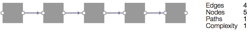
Figure 17: A directed acyclic graph comprised of a single path, which gives it a cyclomatic complexity of one.
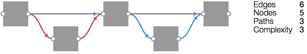
Figure 18: A graph with the same number of nodes as in figure 17 but with three distinct paths (each colour coded). This graph therefore has a cyclomatic complexity of three.
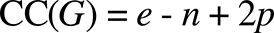
Cyclomatic complexity is a core software engineering metric for measuring code structure. In technical terms, the cyclomatic complexity is the number of independent paths through a directed acyclic graph (DAG). This can be seen visually in figure 17 & 18. The cyclomatic complexity is typically calculated using Thomas McCabe’s (1976, 314) formula:
Where:
- G: the graph.
- e: number of edges. I count parallel edges between identical nodes (duplicate edges) as a single edge.
- n: number of nodes. I do not count non-functional nodes such as comments in text boxes.
- p: number of independent graphs (parts).
McCabe’s formula assumes the DAG has only one input node and one output node, which is infrequently the case with parametric models. In an appraisal of common modifications to McCabe’s original formula, Henderson-Seller and Tegarden (1994, 263) show that “additional (fictitious) edges” can be introduced to deal with multiple inputs and outputs. Thus the cyclomatic complexity formula becomes:

Which (assuming p to be 1) simplifies to:
Where:
- i: number of inputs (dimensionality).
- u: number of outputs.
The cyclomatic complexity indicates how much work is involved in understanding a piece of code. For instance, the DAG in figure 17 can be understood by reading sequentially along the single path of nodes. But understanding the more complicated DAG in figure 18 requires simultaneously reading through three different paths as they diverge and converge back together. While it may be possible to comprehend how three paths interact, this becomes evermore difficult as the complexity increases. As a result, McCabe (1976, 314) recommends restructuring any code with a cyclomatic complexity greater than ten (an idea I explore further in chapter 6). This limit has been reaffirmed by many studies including the United State’s National Institute of Standards and Technology who write, “the original limit of 10 as proposed by McCabe has significant supporting evidence” (Watson and McCabe 1996, sec. 2.5).
Applying Quantitative Metrics
Quantitative metrics lend themselves to statistical analysis. If a collection of code samples are each quantitatively measured, the measurements can be aggregated together and analysed to help identify general trends in the sampled population. This type of analysis does not appear to have been performed in any previous study on parametric models. As a result, the current understanding of parametric modelling is largely confined to firsthand accounts of working with specific parametric models (referred to in chapter 2.3). This leaves significant gaps in the understanding of parametric modelling and many basic questions – such as what is the average size of a parametric model or how complicated is the typical parametric model – remain unanswered. In the following pages I attempt to answer some of these basic questions and establish baselines for the key quantitative metrics I previously discussed (parts of this study were first published in Davis 2011b and then subsequently in Davis et al. 2011b).
Assembling a representative collection of parametric models is difficult since researchers generally only have access to parametric models created by themselves or their colleagues – a likely reason no previous study has quantitatively analysed a group of parametric models. But recently, with the advent of websites enabling communities of designers to share parametric models publicly, large collections of parametric models have been made available. One such website is McNeel’s Grasshopper online forum (grasshopper3d.com) where, between 8 May 2009 and 22 August 2011, 575 designers shared 2041 parametric models. The models are all created in the Grasshopper modelling environment and tend be either a model a designer is having problems with or a model a designer thinks will solve another’s problem. While this collection is not strictly representative of parametric modelling generally, it is a significant advancement over any previous study to be able to analyse, for the first time, how a large number of designers organise models created in a popular parametric modelling environment.
Method
To analyse the models publicly shared on the Grasshopper forum, I first download the 2041 parametric models. The oldest model was from 8 May 2009 and created with Grasshopper 0.6.12, and the most recent model was from 22 August 2011 and created with Grasshopper 0.8.0050. All the models were uploaded to the forum in the proprietary .ghx file format. I reverse engineered this format and wrote a script that extracted the parametric relationships from each file and parsed them into a directed acyclic graph. Thirty-nine models were excluded in this process, either because the file was corrupted or because the model only contained one node (which distorted measurements like cyclomatic complexity). The graphs of the remaining 2002 models were then each evaluated with the previously discussed quantitative metrics. The measurements were then exported to an Excel spreadsheet ready for the statistical analysis. In the analysis I have favoured using the median since the mean is often distorted by a few large outliers. Each of the key quantitative metrics is discussed below.
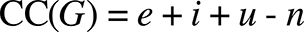
Size
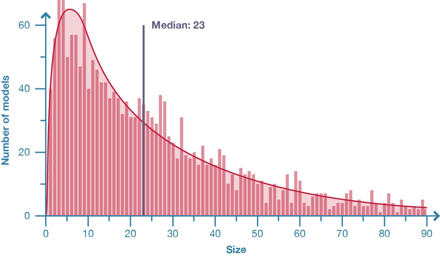
Figure 19: Distribution of model size in population of 2002 parametric models.
The sizes of the 2002 sampled Grasshopper models vary by a number of orders of magnitude; the smallest model contains just two nodes while the largest model contains 2207 nodes (fig. 22). The distribution of sizes has a positive skew (fig. 19) with the median model size being twenty-three nodes. I suspect the skew is partly because many of the models uploaded to the Grasshopper forum are snippets of larger models. The median may therefore be slightly higher in practice. Even with a slightly higher median, the Grasshopper models (including the three models that contain more than one thousand nodes) are very modest compared to those seen in the context of software engineering.
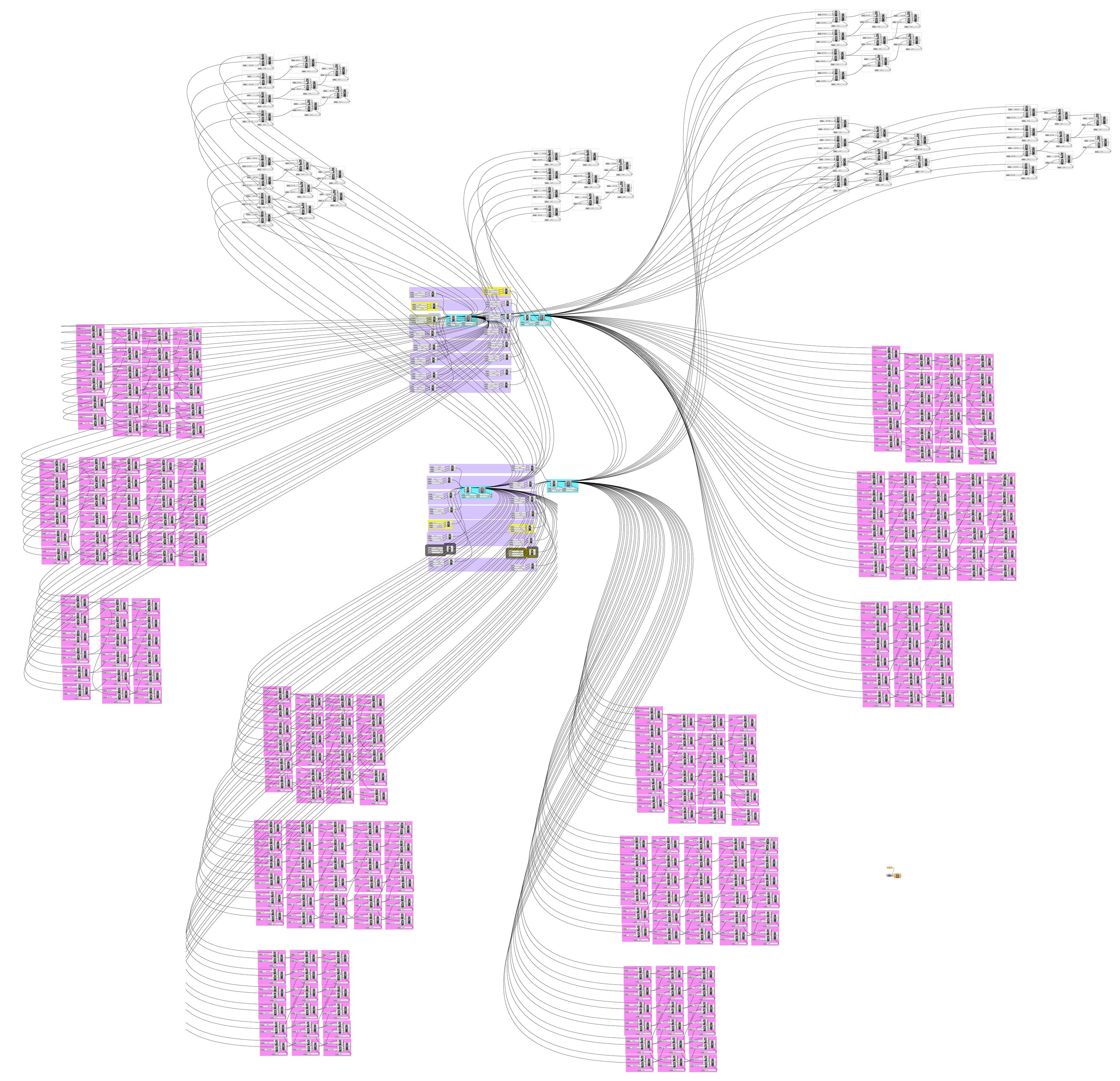
Figure 22: Model-1945, the largest and most complicated model in the sample. With over one thousand inputs, changing any part of the model is a guessing game. I have written previously (Davis 2011b) about how complexity can be reduced in this particular model by refactoring the duplicated elements and condensing the inputs into just twenty critical factors.
Given the numbers of nodes in a model, it is telling to see the typical function of these nodes. I took the 93,530 nodes contained within the 2002 Grasshopper models and ranked them based on function (the top ten are shown in figure 23). The most commonly used node was Number Slider [1], which is a user interface widget for inputting numeric values. Two more interface widgets are also feature highly on the list: Panel [2], which allows users to write and read textual data; and Scribble [8], which lets users explain a DAG by adding text. Also highly ranked were two nodes for managing data arrays: List item [3] and Series [9]. The fourth, fifth, and sixth most popular nodes are all ways of inputting geometry and managing the flow of data. The most popular node with a geometric function is Move [7], which is followed by Point XYZ [10]. In fact, only six of the twenty-five most popular nodes are geometric operations. This demonstrates that parametric modelling, at least within Grasshopper, is as much about inputting data, managing data, and organising the graph as it is about modelling geometry.
Figure 23: Table of the most commonly used node types. These ten node types account for 40% of the 93,530 nodes contained within the 2002 sampled models.
Dimensionality
Figure 20: Distribution of model dimensionality in population of 2002 parametric models.
The vast majority of models have a similar dimensionally; 75% possess between one and eleven inputs with the median being six inputs (fig. 20). Seventeen outliers have more than one hundred inputs and the most extreme model contains 1140 inputs. When examining the models with a high dimensionality, it is strikingly difficult to understand what each input does and even more difficult to change the inputs meaningfully en masse (often the only way is to guess and check). I suspect the comparatively low dimensionality shown in the vast majority of models may be because designers can only comfortably manipulate a few parameters at a time. Therefore, while parameters are a key component of parametric modelling (some would say the defining component: see chap. 2.1) the majority of designers use parameters sparingly in their models.
Cyclomatic Complexity
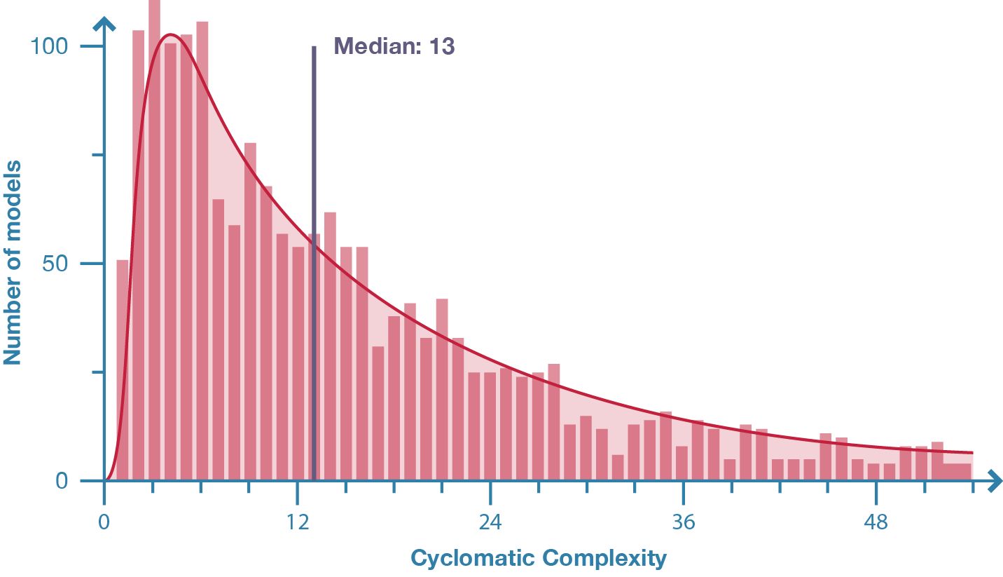
Figure 21: Distribution of model cyclomatic complexity in population of 2002 parametric models.
There is a high variance in the cyclomatic complexity of the sampled models. The median complexity is thirteen (fig. 21) but the range extends from simple models with a complexity of just one, to extremely complex models with a complexity of 1566 (fig. 22). Within this variance, 60% of models have a complexity greater than ten – the limit McCabe (1976, 314) suggested. The differences between complex and simple models are visually apparent in figure 24 where the two extremes are displayed side-by-side. In figure 24, the simple models have orderly chains of commands while the models with a higher cyclomatic complexity have interwoven lines of influence that obfuscate the relationships between nodes. This seems to indicate that cyclomatic complexity is effective in classifying the complexity of a parametric model.
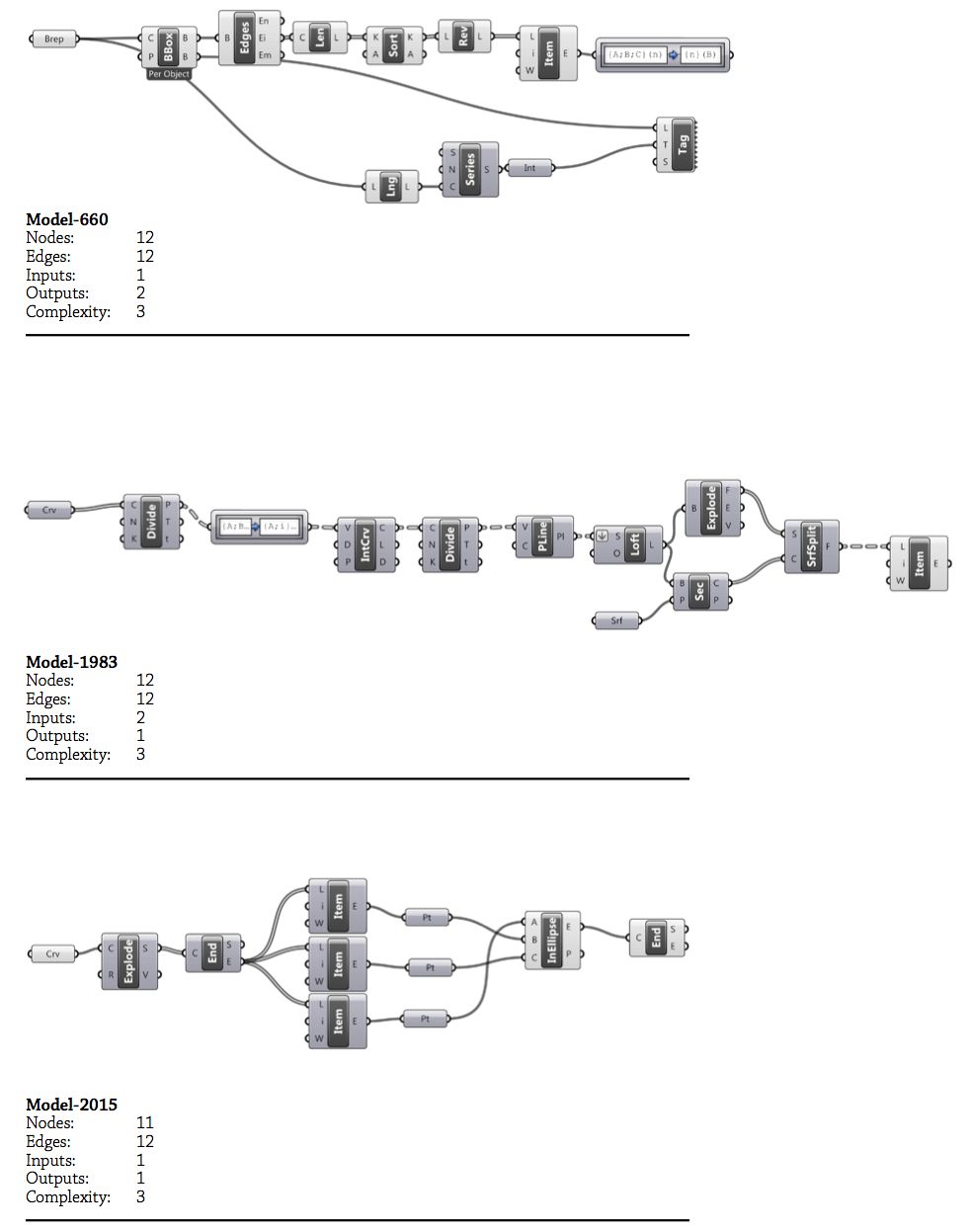
Figure 24: A comparison of models with different cyclomatic complexities. All six models are of a similar size and fairly representative of other models with equivalent complexities. Top: three simple models each with a cyclomatic complexity of three. Bottom: three slightly more complicated models with a cyclomatic complexity of either nine or ten.
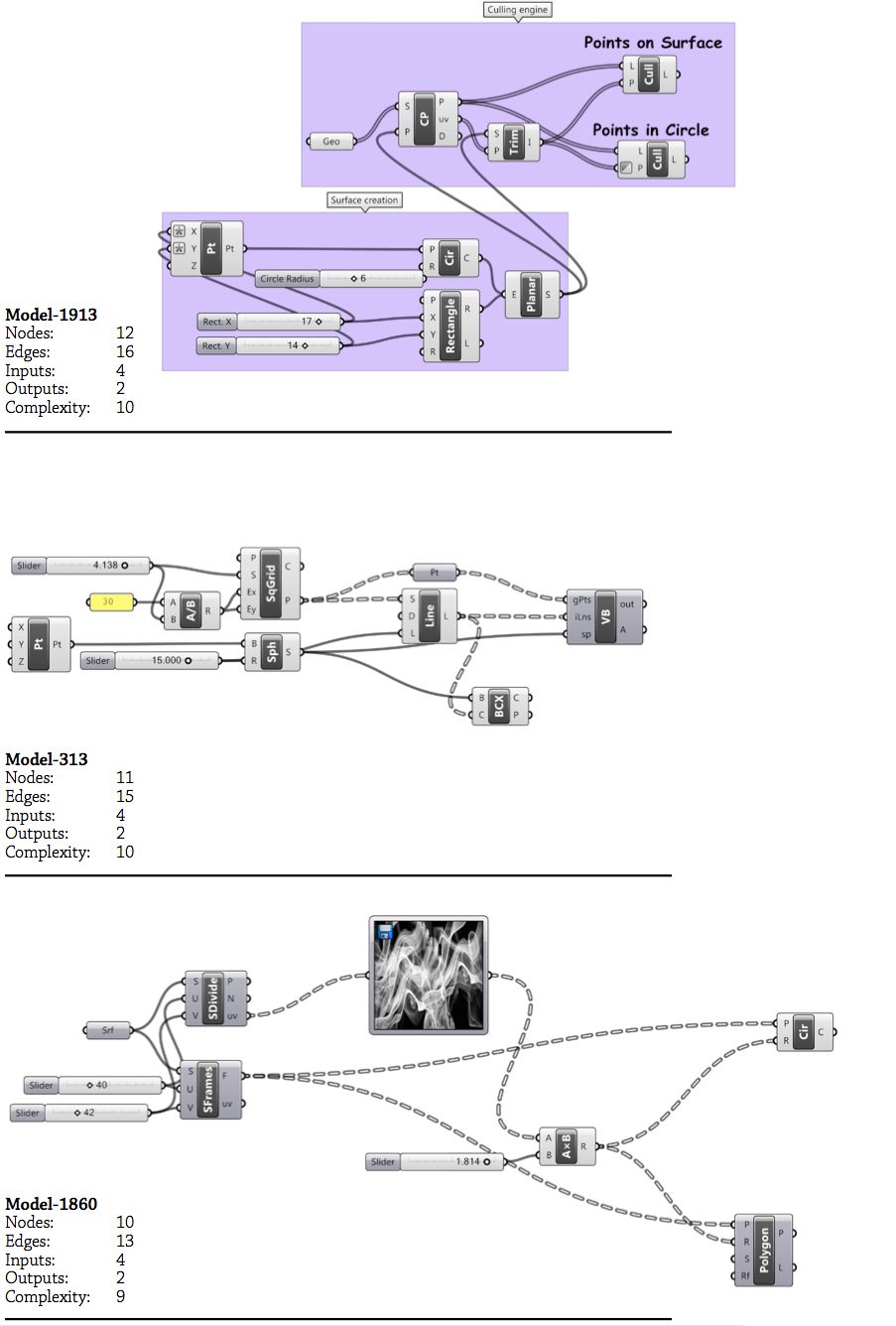
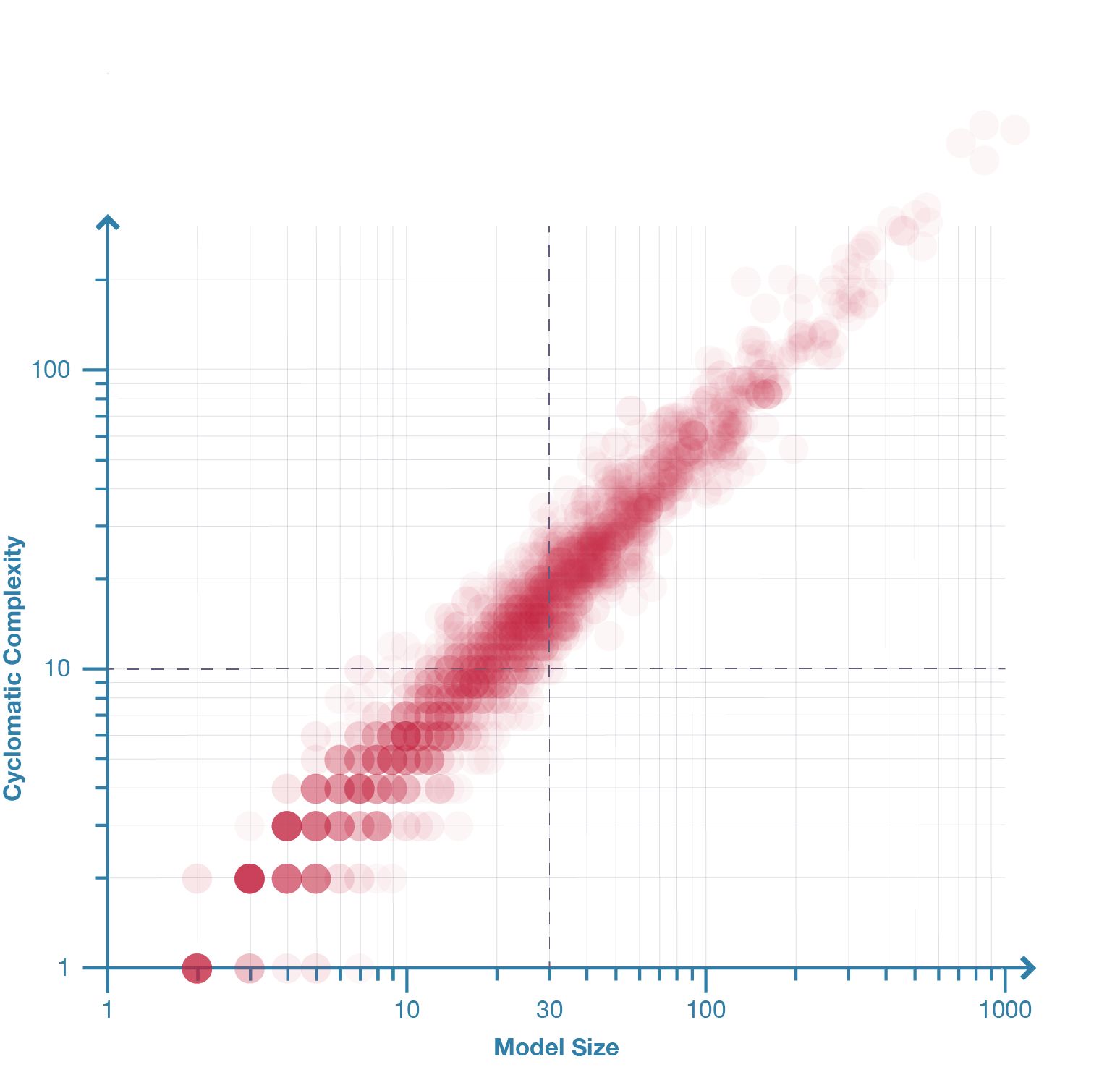
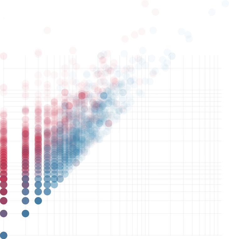
Figure 25: Model complexity plotted against size for 2002 parametric models. The distribution shows a strong correlation between size and complexity (r=0.98). The graph also shows that for models with more than thirty nodes it is inevitable they have a cyclomatic complexity greater than ten.
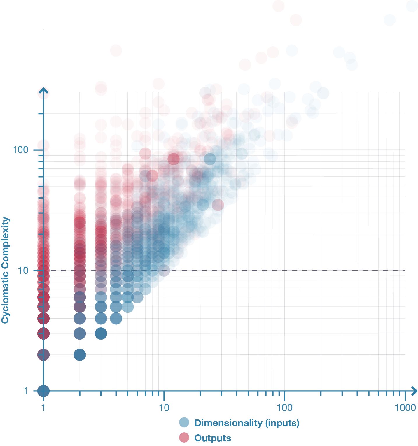
Figure 26: Blue: Model complexity plotted against dimensionality for 2002 parametric models. Red: Model complexity plotted against the number of outputs for 2002 parametric models. The distribution shows that the number of model outputs has little bearing on complexity (r=0.71) since for any given number of outputs there are a range of complexities associated (the vertical spread of red dots). In comparison, the number of inputs has a stronger (r=0.91) relationship to model complexity (the blue dots are more linear and less vertically spread).
A model’s cyclomatic complexity and size are strongly correlated (r=0.98;2 fig. 25). This correlation is significant because it indicates that while a parametric model can theoretically be both large and simple, in actuality, large models tend to be complex (all the models with more than thirty nodes had a cyclomatic complexity greater than McCabe’s limit of ten). A similar correlation exists in software engineering. One such example is van der Meulen and Revilla’s (2007, 206) survey of fifty-nine textual programs that found cyclomatic complexity and LOC to have a correlation of r=0.95. This correlation suggests that complexity is an inevitable by-product of size in both software engineering and parametric modelling. Similar relationships exist for a model’s dimensionality (r=0.91) and outputs (r=0.71), although neither correlates with complexity to the same degree as a model’s size (fig. 25 & 26).
Learning from Quantitative Data
This study is an important first step towards understanding the properties and variations of a typical parametric model. The 2002 Grasshopper models surveyed show that parametric models are generally small and complex. The average model contains twenty-three nodes and even the largest models, with just over one thousand nodes, are modest in the context of software engineering. The size of the model is highly correlated with the model’s complexity, which tends to be very high overall. While one may intuitively expect that the majority of a parametric model consists of parameters and geometry, this study shows that organising the graph and managing data are often the most common components of parametric models created in Grasshopper. Parameters tend to be used surprisingly sparingly, with the vast majority of models only containing between one and eleven parameters.
Another important outcome from this survey is the validation of the quantitative metrics. The study demonstrates that nodes are a good proxy for a model’s size and that the dimensionality can reveal unintuitive insights regarding the use of parameters in parametric models. Furthermore, the cyclomatic complexity seems to fairly accurately differentiate between simple and complex models. However, despite the validation of these quantitative metrics, they still only tell a narrow part of a model’s story; a story that can be further triangulated with qualitative measures.
4.4 – Qualitative Flexibility
Many aspects of parametric flexibility elude quantitative measurement. While it is useful to know the size of a model or the complexity of a model, by themselves, these measurements give an incomplete picture. Bertrand Meyer (1997, 3) argues, in his seminal book Object-Oriented Software Construction, “software quality is best described as a combination of several factors.” Meyer (1997, chap. 1) spends the first chapter of his book expounding the following ten factors of “software quality”:
- Correctness: ability of software products to perform their exact tasks, as defined by their specification.
- Robustness: the ability of software systems to react appropriately to abnormal conditions.
- Extendability: the ease of adapting software products to changes of specification.
- Reusability: the ability of software elements to serve for the construction of many different applications.
- Compatibility: the ease of combining software elements with others.
- Efficiency: the ability of a software system to place as few demands as possible on hardware resources.
- Portability: the ease of transferring software products to various hardware and software environments.
- Ease of use: the ease with which people of various backgrounds and qualifications can learn to use software products and apply them to solve problems.
- Functionality: the extent of possibilities provided by a system.
- Timelessness: the ability of a software system to be released when or before its users want it.
While other authors have constructed similar lists of software quality (Meyer 1997, 19-20), Meyer’s list holds significant cachet in software engineering because it belongs to one of the most cited books in computer science.3 There are notable correlations between Meyer’s list and the ISO/IEC standard for Software Product Quality (ISO 2000), with Meyer’s efficiency, portability, ease of use, and functionality being word-for-word identical to the ISO categories. In this thesis I take the factors Meyer identifies as being crucial to software quality and I use them as a structure for qualitative evaluations of parametric models. In particular, I make reference to Meyer’s concepts of correctness [1], extendability [3], reusability [4], efficiency [6], ease of use [8], and functionality [9], which I will now briefly explain in more detail.
Correctness
Correctness concerns whether software does what is expected. In some circumstances correctness is obvious; if you create a parametric model to draw a cube, the model is correct if it draws one. But in most circumstances correctness is non-trivial since it can be difficult to determine what is expected and to ensure this happens through a range of input parameter values. Software engineers have developed a range of methods for ascertaining whether software is correct – unit testing being one notable example. While I suspect architects would benefit from adopting these practices, this is a large area of research outside the scope of my thesis (as discussed in chapter 3). For the remainder of this thesis I have used correctness to denote that a parametric model is free from any major defects; it is not creating spheres when it should be creating cubes.
Extendability
Extendability is essentially a synonym for flexibility; the ease with which software adapts to changes. Meyer (1997, 7) says extendability correlates with size, since “for small programs change is usually not a difficult issue; but as software grows bigger, it becomes harder and harder to adapt.” This notion corresponds to what other authors have written about the software crisis (see chap. 3.1) and it corresponds to the relationships between software size and cyclomatic complexity that I have empirically shown. Meyer (1997, 7) goes on to argue that extendability can be improved by ensuring the code has a “simple architecture,” which can be achieved by structuring the code with “autonomous modules.” While I explore extendability throughout this thesis, I pay particular attention to the structure of parametric models in chapter 6.
Reusability
Reusability pertains to how easily code can be shared, either in part or in whole. Meyer (1997, 7) notes that “reusability has become a pressing concern” of software engineers. As I have shown in chapter 2.3, the reusability of parametric models is also a concern of many architects.
Efficiency
Efficiency describes how much load a program places on hardware. This is particularly pertinent to architects because a program’s efficiency helps determine its latency, which, in turn, affects change blindness (see chap. 2.3). In extreme cases the model’s efficiency may even determine its viability, since certain geometric calculations are so computationally demanding that inefficient models can slow them to the point of impracticality. However, Meyer (1997, 9) tells software engineers “do not worry how fast it is unless it is also right” and warns, “extreme optimizations may make the software so specialized as to be unfit for change and reuse.” Thus, efficiency can be important but it needs to be balanced against other attributes like correctness and reusability.
Ease of Use
Ease of use is fairly self-explanatory. For architects, ease of use applies to both the modelling environment and the model. A modelling environment’s ease of use concerns things like user interface and modelling workflow. A designer familiar with a modelling environment will tend to find it easier to use, which impacts how fast they can construct models (construction time) and how competently they can make changes (modification time). In addition to the modelling environment being easy to use, the model itself needs to be easy to use. I have spoken previously about the importance of dimensionality and complexity when it comes to understanding and changing a model. Meyer (1997, 11) echoes this point, saying a “well thought-out structure, will tend to be easier to learn and use than a messy one.”
Functionality
Functionality to Meyer (1997, 12) denotes “the extent of possibilities provided by a system.” Like ease of use, functionality is applicable to both the modelling environment and the model. The key areas of functionality in a modelling environment include the types of geometry permissible, the types of relationships permissible, and the method of expressing relationships. Modelling operations that are easy to implement in one environment may be very difficult (or impossible) in another due to variations in functionality. Likewise, changes easily permissible in one environment may be challenging in another. Therefore, the functionality of a modelling environment helps determine the functionality of the parametric model. This is a determination that often comes early in the project since changing the modelling environment mid-project normally means starting again.
Using Qualitative Metrics
All of the qualitative metrics require some form of consideration and judgment in their application. Some have established protocols of observation – for example, there are well-researched ways to conduct usability studies in order to analyse ease of use. Other qualitative assessments can be logically deduced through comparisons – for example, the functionality of a modelling environment can be evaluated by comparing its features to those of other environments. But other attributes, like extendability, fall upon expert judgment to analyse. None of these are definitive measurements, for even the quantitative measurements are distorted by what they cannot measure. However, the qualitative measurement do provide a vocabulary of attributes to begin capturing the qualities of a parametric model.
4.5 – Conclusion
Meyer (1997, 15) stresses that software metrics often conflict. Each metric offers one perspective, and improvements in one perspective may have negative consequences in another. For example, making a model more efficient may make it less extendible, and making a model more reusable may harm the latency. Furthermore, measured improvements may not necessarily manifest in improved flexibility since flexibility is partly a product of chance and circumstance; an apparently flexible model (one that is correct, easy to use, and with a low cyclomatic complexity) can stiffen and break whilst a seemingly inflexible model may make the same change effortlessly. This uncertainty makes any single measure of flexibility – at best – an estimation of future performance.
To help mitigate the biases of any single metric, I plan to aggregate a triangulated perspective of the case studies using a variety of metrics. In this chapter I have discussed a range of metrics applicable to parametric modelling: from quantitative metrics to measure time, size, and complexity; to qualitative metrics to begin discussing qualities like correctness, functionality, and reusability. By gathering these measurements together in this chapter I have begun to articulate a vocabulary for discussing parametric models; a vocabulary that goes beyond the current binaries of failure and success. Using parts of this vocabulary I have been able to analyse, for the first time, a large collection of parametric models in order to get a sense of the complexity, composition, and size of a typical parametric model. This demonstrates the viability of quantitatively measuring qualities like cyclomatic complexity but also demonstrates why quantitative metrics alone are not enough to observe the case studies.
In addition to the suite of metrics, this chapter has also identified three case studies to test various aspects of the software engineering body of knowledge. The case studies have been selected not because the cases are necessarily representative of challenges architects typically encounter, but because cases provide the best opportunity to learn about these challenges. Each of the following three chapters contains one of these case studies and makes use of a variety of the metrics discussed in this chapter.
Thesis Navigation
- Return to table of contents
- Goto previous chapter
- Goto next chapter
- Download entire thesis as PDF (30mb)
Footnotes
1:The ISO/IEC 9126 standard has metrics for everything from how easy the help system is to use, to how long the user waits while the code accesses an external device.
2:r is Pearson’s coefficient. A value of 1 indicates that two variables are perfectly correlated (all sampled points fall on a line), a value of 0 indicates that two variables are not not correlated in any way (one does not predict the other), and a negative value indicates an inverse correlation.
3:CiteSeer (2012) say Object-Oriented Software Construction is the sixty-second most cited work in their database of over two million computer science papers and books.
Bibliography
Aberdeen Group. 2007. “The Design Reuse Benchmark Report: Seizing the Opportunity to Shorten Product Development.” February. Boston: Aberdeen Group.
Boehm, Barry. 1976. “Software Engineering.” IEEE Transactions on Computers 25 (12): 1226-1241.
Brooks, Frederick. 1975. The Mythical Man-month : Essays on Software Engineering. Anniversary edition. Boston: Addison-Wesley.
Card, Stuart, George Robertson, and Jock Mackinlay. 1991. “The Information Visualizer, an Information Workspace.” In Reaching Through Technology: Proceedings of the SIGCHI Conference on Human Factors in Computing Systems, 181–188. New Orleans: Association for Computing Machinery.
Christensen, Henrik. 2010. Flexible, Reliable Software: Using Patterns and Agile Development. Boca Raton: Chapman & Hall/CRC.
CiteSeer. 2012. “Most Cited Computer Science Articles.” Published 20 May. http://citeseerx.ist.psu.edu/stats/articles.
Creswell, John, and Vicki Clark. 2007. Designing and Conducting: Mixed Methods Research. Thousand Oaks: Sage.
Davis, Daniel. 2011b. “Datamining Grasshopper.” Digital Morphogenesis. Published 20 September. http://www.nzarchitecture.com/blog/index.php/2011/09/20/datamining-grasshopper/.
Davis, Daniel, Jane Burry, and Mark Burry. 2011b. “Understanding Visual Scripts: Improving collaboration through modular programming.” International Journal of Architectural Computing 9 (4): 361-376.
Dijkstra, Edsger. 1970. Notes on Structured Programming. Second Edition. Eindhoven: Technological University of Eindhoven.
El Emam, Khaled, Saïda Benlarbi, Nishith Goel, and Shesh Rai. 2001. “The Confounding Effect of Class Size on the Validity of Object-Oriented Metrics.” IEEE Transactions on Software Engineering 27 (7): 630-650.
Erhan, Halil, Robert Woodbury, and Nahal Salmasi. 2009. “Visual Sensitivity Analysis of Parametric Design Models: Improving Agility in Design.” In Joining Languages, Cultures and Visions: Proceedings of the 13th International Conference on Computer Aided Architectural Design Futures, edited by Temy Tidafi and Tomás Dorta, 815–829. Montreal: Les Presses de l'Université de Montréal.
Evans, David, and Paul Gruba. 2002. How to Write a Better Thesis. Second edition. Melbourne: Melbourne University Press.
Henderson-Sellers, Brian, and David Tegarden. 1994. “The Theoretical Extension of Two Versions of Cyclomatic Complexity to Multiple Entry/exit Modules.” Software Quality Journal 3 (4): 253–269.
Hilburn, Thomas, Iraj Hirmanpour, Soheil Khajenoori, Richard Turner, and Abir Qasem. 1999. A Software Engineering Body of Knowledge Version 1.0. Pittsburgh: Carnegie Mellon University.
ISO (International Organisation for Standards). 2000. Information Technology: Software product quality – Part 1: Quality model. ISO/IEC 9126. New York: American National Standards Institute.
Ko, Andrew. 2010. “Understanding Software Engineering Through Qualitative Methods.” In Making Software: What Really Works, and Why We Believe It, edited Andy Oram and Greg Wilson, 55–64. Sebastopol: O’Reilly.
Lincke, Rudiger, and Welf Lowe. 2007. Compendium of Software Quality Standards and Metrics. Version 1.0. Published 3 April. http://www.arisa.se/compendium/.
McCabe, Thomas. 1976. “A Complexity Measure.” IEEE Transactions on Software Engineering 2 (4): 308-320.
McConnell, Steven. 2006. Software Estimation: Demystifying the Black Art. Redmond: Microsoft Press.
Menzies, Tim, and Forrest Shull. 2010. “The Quest for Convincing Evidence.” In Making Software: What Really Works, and Why We Believe It, edited Andy Oram and Greg Wilson, 3-11. Sebastopol: O’Reilly.
Meyer, Bertrand. 1997. Object-Oriented Software Construction. Second edition. Upper Saddle River: Prentice Hall.
Miller, Robert. 1968. “Response Time in Man-Computer Conversational Transactions.” In Proceedings of the AFIPS Fall Joint Computer Conference, 267–277. Washington, DC: Thompson.
Nasirova, Diliara, Halil Erhan, Andy Huang, Robert Woodbury, and Bernhard Riecke. 2011. “Change Detection in 3D Parametric Systems: Human-Centered Interfaces for Change Visualization.” In Designing Together: Proceedings of the 14th International Conference on Computer Aided Architectural Design Futures, edited by Pierre Leclercq, Ann Heylighen, and Geneviève Martin, 751–764. Liège: Les Éditions de l’Université de Liège.
PTC (Parametric Technology Corporation). 2008. “Explicit Modeling: What To Do When Your 3D CAD Productivity Isn’t What You Expected.” White-paper. Needham: Parametric Technology Corporation.
Schön, Donald. 1983. The Reflective Practitioner: How Professionals Think in Action. London: Maurice Temple Smith.
Smith, Rick. 2007. “Technical Notes From Experiences and Studies in Using Parametric and BIM Architectural Software.” Published 4 March. http://www.vbtllc.com/images/VBTTechnicalNotes.pdf.
Stake, Robert. 2005. “Qualitative Case Studies.” In The SAGE Handbook of Qualitative Research, edited Norman Denzin and Yvonnas Lincoln, 443-466. Third edition. Thousand Oaks: Sage.
Watson, Arthur, and Thomas McCabe. 1996. Structured Testing: A Testing Methodology Using the Cyclomatic Complexity Metric. Gaithersburg: National Institute of Standards and Technology.
Woodbury, Robert. 2010. Elements of Parametric Design. Abingdon: Routledge.
van der Meulen, Meine, and Miguel Revilla. 2007. “Correlations Between Internal Software Metrics and Software Dependability in a Large Population of Small C/C++ Programs.” In Proceedings of the 18th IEEE International Symposium on Software Reliability, 203–208. Sweden: IEEE Computer Society Press.
Illustration Credits
- Figure 17 – Daniel Davis
- Figure 18 – Daniel Davis
- Figure 19 – Daniel Davis
- Figure 20 – Daniel Davis
- Figure 21 – Daniel Davis
- Figure 22 – Model by Ryan Hernandez, http://www.grasshopper3d.com/forum/topics/deforming-circles
- Figure 23 – Daniel Davis
- Figure 24 – Model-313 by Andy VanMater, http://www.grasshopper3d.com/forum/topics/curvebrep-intersection-errors; Model-660 by Peter Kluck, http://www.grasshopper3d.com/forum/topics/structural-profile-length; Model-1860 by Isak Bergwall, http://www.grasshopper3d.com/forum/topics/need-som-help-with-circles; Model-1913 by Chris Tietjen, http://www.grasshopper3d.com/forum/topics/how-can-i-project-objectlike; Model-1983 by Tijl Uijtenhaak, http://www.grasshopper3d.com/forum/topics/trouble-with-surface-split; Model-2015 by Rassul Wassa, http://www.grasshopper3d.com/forum/topics/create-inellipse-for-a
- Figure 25 – Daniel Davis
- Figure 26 – Daniel Davis