
Drawing a hyperboloid seems like a reasonably straightforward task. In a world where architects are accustomed to creating complicated, non-uniform, free-form surfaces, the hyperboloid is a relatively regular shape. It seems trivial. Already you've probably thought of three ways to draw a hyperboloid. I can tell you: they are all wrong.
For the past five years I've been drawing hyperboloids. Working as an assistant to Mark Burry on Antoni Gaudí’s Sagrada Família, I've drawn hyperboloids over and over. I've never quite managed to draw a totally accurate one in Rhino (often we have to use more sophisticated software like CATIA). My quest to draw the perfect hyperboloid has taken me progressively deeper into the geometry engine underlying NURBs based CAD programs like Rhino. Last month, I finally found a way to draw an accurate hyperboloid.
My hyperboloid drawing method derives from the underlying mathematics of NURBs surfaces. Despite the reliance on NURBs in contemporary architecture, I’ve never read anything about this fundamental geometric formula, much less about how to manipulate this formula to draw accurate shapes. In this post I’ll outline a number of methods for drawing hyperboloids. In the process I’ll expose the mechanisms of NURBs and show how you can take advantage of these formulas to draw mathematically accurate shapes.
1. An intuitive hyperboloid

A hyperboloid can be generated intuitively by taking a cylinder and twisting one end. Twist tight enough and you’ll get two cones meeting at a point. Twist gently and you’ll get a shape somewhere between a cone and a cylinder: a hyperboloid. Depending on how you look at it, it is either a cylinder that flairs outwards or a cone that never quite comes to a point.
The hyperboloid is a doubly ruled surface. That is to say, for any point on the hyperboloid, two perfectly straight lines can be drawn on the surface passing through that point. This is the unique property of doubly ruled surfaces: although they are curved, you can always find a straight line on them.

The interior of the Sagrada Família looks complicated, but if you study the geometry carefully, you'll see that it is composed using a series of mathematical rules. In this case, the ceiling comprises of hyperboloids. The triangular cutouts follow the ruled geometry of the hyperboloids.
Most of my work for Mark Burry on Gaudí’s Sagrada Família involves hyperboloids in some way. Even projects I’ve worked on outside the Sagrada Família (still with Mark), such as the Responsive Acoustic Surface and the Fab Pod, are comprised of hyperboloids. I’ve milled hyperboloids from plywood, I’ve made them with spun metal, 3d printers, and plaster. On my 24th birthday, my girlfriend made me a hyperboloid shaped cake. In this strange way, hyperboloids have become a regular part of what I do.
 is made from hyperboloids positioned to optimise their acoustic properties. Photograph by John Gollings.](/img/20130316_DX_0438-people-variations-R_3523yOYn-1280w.jpeg)
The Fab Pod is made from hyperboloids positioned to optimise their acoustic properties. Photograph by John Gollings.
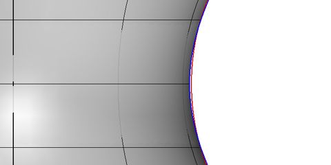
While hyperboloids are easy to explain, they are difficult to draw in Rhino. The easiest way to draw a hyperboloid is to follow the explanation I’ve given above. Draw two offset circles (the two ends of the cylinder), twist one of the circles, draw a line between the circles, and create a revolved surface using that line. The code below shows how to do this. Unfortunately, you often end up with weird artifacts at the neck of the hyperboloid (shown below). This has to do with how the revolved line skews the UV curves of the hyperboloid surface. The construction logic of the hyperboloid doesn't necessarily translate into the computer.
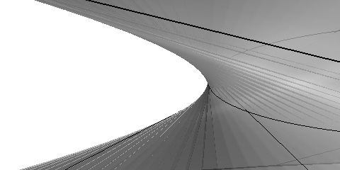
These striations in the neck of the hyperboloid come from the meshing algorithm. The twist makes everything somewhat inaccurate.
# Rhino Python code to make a twisted hyperboloid
import scriptcontext
import Rhino
import math
def get_hyperboloid(radius, twist, depth) :
    """
    Create revolved surface from line between circles.
    """
    top = Rhino.Geometry.Point3d(0,0,depth)
    top = Rhino.Geometry.Plane(top, Rhino.Geometry.Vector3d.ZAxis)
    top = Rhino.Geometry.Circle(top, radius)
    bottom = Rhino.Geometry.Point3d(0,0,-depth)
    bottom = Rhino.Geometry.Plane(bottom, Rhino.Geometry.Vector3d.ZAxis)
    bottom = Rhino.Geometry.Circle(bottom, radius)

    p_top = top.PointAt(0)
    p_bottom = bottom.PointAt(twist)

    line = Rhino.Geometry.Line(p_top, p_bottom)
    axis = Rhino.Geometry.Line(Rhino.Geometry.Point3d(0,0,0), Rhino.Geometry.Point3d(0,0,1))
    hyperboloid = Rhino.Geometry.RevSurface.Create(line, axis)

    return hyperboloid

if __name__=="__main__":
    """
    Generate and bake hyperboloid.
    """
    hyperboloid = get_hyperboloid(2, 2, 1)
    attributes = Rhino.DocObjects.ObjectAttributes()
    scriptcontext.doc.Objects.AddSurface(hyperboloid, attributes)
    scriptcontext.doc.Views.Redraw()
2. A mathematical hyperboloid
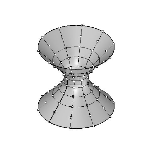
These points were positioned using the hyperboloid formula. The surface was then interpolated through the points to generate the hyperboloid. While the points are accurate, the surface is still not entirely precise.
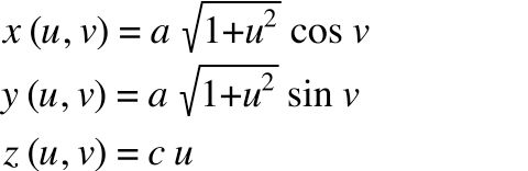
A hyperboloid can also be defined mathematically. The formula for a hyperboloid is:
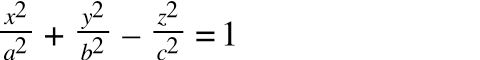
Parameterised, the formula becomes:
Using this formula, we can generate any point on the hyperboloid. If we generate enough points, we can create an interpolated surface through the points.
# Rhino Python code to make an interpolated hyperboloid
import scriptcontext
import Rhino
import math

def get_hyperboloid(a, b, c, depth) :
    """
    Create revolved surface from hyperbola.
    Scale to match proportions of hyperboloid.
    """
    detail_u = 10
    detail_v = 10

    pts = list()

    for u in range(int(detail_u)):
        for v in range(int(detail_v)):
            u_normal = ((depth * 2 * u / (detail_u - 1)) - depth) / c
            v_normal = 2 * math.pi * v / (detail_v)

            x = a * math.sqrt(1 + u_normal**2) * math.cos(v_normal)
            y = b * math.sqrt(1 + u_normal**2) * math.sin(v_normal)
            z = c * u_normal

            p = Rhino.Geometry.Point3d(x, y, z)

            pts.append(p)

    hyperboloid = Rhino.Geometry.NurbsSurface.CreateThroughPoints(pts, detail_u, detail_v, 3, 3, False, True)
    return hyperboloid

if __name__=="__main__":
    """
    Generate and bake hyperboloid.
    """
    hyperbola = get_hyperboloid(1, 2, 1, 6)
    attributes = Rhino.DocObjects.ObjectAttributes()
    scriptcontext.doc.Objects.AddSurface(hyperbola, attributes)
    scriptcontext.doc.Views.Redraw()
For a number of years this was the method I used to draw hyperboloids. From a distance it looks good, but if you examine the surface closely you’ll notice some slight inaccuracies. The points are in the right place, but the parts in-between – the parts that were interpolated – are sometimes too flat or too bent. This is because the interpolated curve is following the NURBs formula rather than the hyperboloid formula. The curve passes through all the points we defined but the curve is not following the mathematical formula we used.
In a section through a hyperboloid you can see the difference between an interpolated hyperboloid (red) and an accurate one (blue). The difference is visually minor but fairly severe in a practical sense.
The accuracy can be somewhat improved by increasing the number of points (which effectively reduces the distance of interpolation). Unfortunately, increasing the points also increases the computational complexity of the surface. At a certain density, the surfaces become unmanageable. This can be somewhat mitigated by using fewer points in the flatter areas of the hyperboloid and more points in the curved section. Even then, the inaccuracy is only reduced and never eliminated. There will always be problems with the surface.
3. A BIM hyperboloid
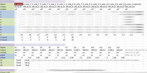
Excel spreadsheet containing names and positions of hyperboloids. Some data has been obscured.
I got around the interpolation problem by bypassing the Rhino geometry engine and creating my own specially for hyperboloids. Rather than drawing the hyperboloids in Rhino, I would store the shape of the hyperboloids in a spreadsheet. If I needed view the hyperboloids, I would draw them in Rhino, but if I needed to manipulate the hyperboloids, I would do it mathematically through code. For example, instead of relying on Rhino’s intersection function to find the junction between two hyperboloids, I would mathematically calculate where this intersection occurred based on the data from the spreadsheet. The results were perfect, the interface was clunky, and the mathematics was non-trivial. In my thesis I wrote about finding the intersections between hyperboloids on the Fab Pod, the equation looked like this:

4. A NURBs hyperboloid
Recently on the Sagrada Família we once again ran into the problem with the accuracy of the hyperboloids in Rhino. I began investigating how Rhino drew native elements like circles, which didn't seem to suffer from any interpolation problems. They were always perfect. My initial assumption was that Rhino handled these native elements differently to other free-form NURBs curves. It seemed that Rhino was somehow using the formula for the circle instead of the NURBs formula. I was half-right. Rhino does use the formula for the circle but only via the NURBs formula. In other words, Rhino manipulates the inputs to the NURBs formula in such a way that it becomes the circle formula. On Wikipedia there is even an example of how to draw a perfect circle using NURBs.
](/img/Screen-Shot-2014-09-01-at-4.19.37-pm1-jPGGXmyVPD-480w.jpeg)
Location and weights of control points for a perfect NURBs circle. As explained in: http://en.wikipedia.org/wiki/Non-uniform_rational_B-spline
As an example, I'll show you how to derive the points and weights needed to draw a hyperboloid using NURBs. First you need to see the NURBs formula, which looks a bit crazy:
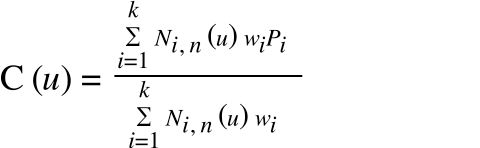
Where:
- C is the point being calculated,
- u is the location of the calculated point,
- P is a control point,
- w is the corresponding weight,
- k is the number of control points,
- N is the b-spline basis function,
- And n is the degree of the curve.
The NURBs formula is a general version of the Bézier formula. If the points and weights of a Bézier curve are put into the NURBs formula, it will draw an identical shape. The only difference between NURBs curves and Bézier curves is that NURBs curves can have additional knots (essentially kinks) whereas Bézier curves can only draw continuous shapes. You'll notice that the Bézier formula is therefore slightly more simple than the NURBs formula:
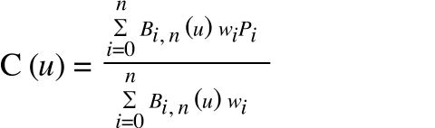
Where B is the Bernstein polynomial.
Since the hyperboloid is a continuous shape, the Bézier formula can be used to derive the points and weights needed to draw a hyperboloid. Before drawing the 3d hyperboloid, we will first draw the 2d profile: a hyperbola. There is a hyperbola tool in Rhino but there isn't any way to generate a hyperbola algorithmically. You could draw one using an interpolated curve, but as I've shown above, this will produce inaccurate results. The only way to draw a hyperbola accurately is to turn the formula for the Bézier curve into the formula for a hyperbola.
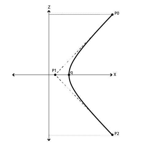
A hyperbola drawn on the XZ plan. To draw this hyperbola we need to calculate P0, P1, P2, and q.
The hyperbola formula looks like this (note that I'm drawing the hyperbola on the XZ plane just so the hyperbola lines up with the hyperboloid formula given above):
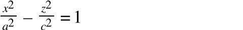
To turn the Bézier formula into the hyperbola formula, we first need to know the degree of curve. Hyperbolas are quadratic since the highest order is two (everything is to the power of two). Based on the Bézier formula above, the Bernstein polynomial for a quadratic curve is:
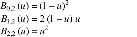
These Bernstein polynomials can be inputted into the Bézier formula, which results in:
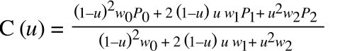
All of a sudden there are only six unknowns in the Bézier formula: _P_0, _P_1, _P_2, & their corresponding weights. We just have to find these six values such that the formula equals the hyperbola formula (see diagram above to get a sense for how these points relate to the hyperbola).
One property of Bézier curves is that the curve always passes through the start and end points. This means the weights of these points doesn't matter, so we can set _w_0 and _w_2 to 1. This also means that _P_0 and _P_2 must be a point on the hyperbola. Using the hyperbola formula, and setting P0 at an arbitrary height (h) on the z-axis, _P_0 becomes:
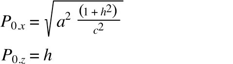
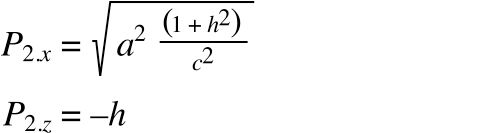
Where h is the height of the hyperbola. For simplicity sake, we will make _P_2 the mirror image of _P_0:
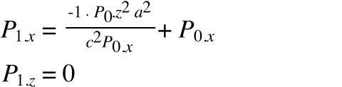
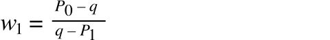
The only variables outstanding are _P_1 and _w_1. We know that _P_1 lies on the x-axis, so _P_1.z must equal zero. We also know that the ends of a Bézier curve are always tangential to the control points. In other words, the line between _P_1 and _P_0 is tangental to the hyperbola at _P_0.
The tangent of a hyperbola is:
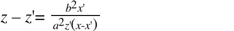
Where:
- x, z is the point on the tangent (_P_1),
- and x', z' is the point on the hyperbola we are calculating the tangent for (_P_0).
Since P0 is a point on the hyperbola that _P_1 is tangental to, we can use _P_0 for x' & z'. And since _P_1 lies on the x-axis, _P_1.z must be zero. Therefore, all we need to solve for is x. Putting these variables into the formula above and rearranging gives the location of _P_1 relative to _P_0:
All that is left to calculate is _w_1. Since the hyperbola is symmetrical, we know the hyperbola will intersect with the x-axis at the apex of the curve (point q). Point q lies on the x-axis, so z=0 for point q. Putting z=0 into the hyperbola formula gives the location of point q as:
Point q is the middle of the hyperbola. In the Bézier formula, this occurs when u=0.5. Putting u=0.5 into the Bézier formula results in:
Simplifying and replacing the values we have calculated above (wo = 1, w1 = 2, P2 = P0 [which happens in the x dimension], and C(0.5) for q) gives:
Multiplying the denominator and numerator by two:
Rearranging:
And with that, we have all the variables for defining a hyperbola (_P_0, _P_1, _P_2, _w_0, _w_1, _w_2). Putting this all into Rhino Python, you end up with the code below.
#Rhino Python code to make an accurate hyperboloid
import scriptcontext
import Rhino
import math

def get_hyperbola(a, c, h) :
    """
    Draws a hyperbola on the XZ plane, centred at 0,0,0.
    """

    p0 = Rhino.Geometry.Point3d(0, 0, 0)
    p1 = Rhino.Geometry.Point3d(0, 0, 0)
    p2 = Rhino.Geometry.Point3d(0, 0, 0)
    q = Rhino.Geometry.Point3d(0, 0, 0)

    p0.X = math.sqrt(a**2 * (1 + (h**2 / c**2)))
    p0.Z = h

    p1.X = (-1 * p0.Z**2 * a**2) / (c**2 * p0.X) + p0.X
    p1.Z = 0

    p2.X = p0.X
    p2.Z = -h

    q.X = a
    q.Z = 0

    w1 = (p0.X-q.X) / (q.X-p1.X)

    points = [p0, p1, p2]
    hyperbola = Rhino.Geometry.NurbsCurve.Create(False, 2, points)
    hyperbola.Points.SetPoint(1, Rhino.Geometry.Point4d(p1.X, p1.Y, p1.Z, w1))

    return hyperbola

def get_hyperboloid(a, b, c, depth) :
    """
    Create revolved surface from hyperbola.
    Scale to match proportions of hyperboloid.
    """
    hyperbola = get_hyperbola(a, c, depth)
    axis = Rhino.Geometry.Line(Rhino.Geometry.Point3d(0,0,0), Rhino.Geometry.Point3d(0,0,1))
    hyperboloid = Rhino.Geometry.RevSurface.Create(hyperbola, axis)

    y_factor = float(b) / float(a)
    scale = Rhino.Geometry.Transform.Scale(Rhino.Geometry.Plane.WorldXY, 1, y_factor, 1)
    hyperboloid = hyperboloid.ToNurbsSurface()
    hyperboloid.Transform(scale)

    return hyperboloid

if __name__=="__main__":
    """
    Generate and bake hyperboloid.
    """
    hyperboloid = get_hyperboloid(1, 2, 1, 6)
    attributes = Rhino.DocObjects.ObjectAttributes()
    scriptcontext.doc.Objects.AddSurface(hyperboloid, attributes)
    scriptcontext.doc.Views.Redraw()
This code produces the hyperboloid below. It is a hyperboloid defined by only twenty-four control points, all weighted perfectly to give an absolutely precise hyperboloid. The geometry is lightweight, accurate, and splits cleanly with ruled lines. It has taken me a long time to get to this stage, but I finally feel like I understand – and can therefore control - the equations underlying software like Rhino. Hopefully this post has given you some insight into the underlying equations of CAD software and how they can be manipulated. And if not, hopefully you’ve at least learnt the many ways to draw a hyperboloid.
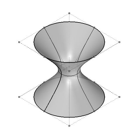
A mathematically accurate hyperboloid defined from just 24 control points.
All code in this post licensed under Creative Commons attribution.
Maher
Loved the article! Well-explained and clearly written. Curious about what CATIA would generate. Did you run any tests?
Daniel
Hey Mahar, I haven't done an explicit test but on occasion I have ended up in a situation where the Rhino model doesn't quite match the CATIA model. This is to do with how I was modeling geometry in Rhino. CATIA has a lot of inbuilt checks and balances that ensures the integrity of the surfaces, so we haven't experienced any accuracy problems in CATIA.
Nick Aplin
I hope to make a planter in which to grow 'enriched' geraniums. what I imagine is one about 16 in. in diameter top and bottom and about 10 to 12 in. high with the minimum diameter being perhaps 14 in. (the shape to be a one sheeted hyperboloid)
I hope to create a frame using small pieces of wood, around which to wrap fabric and then to use as a mould for possibly clay or plaster of paris ...??
Any suggestions will be appreciated ... Thanks!
Daniel
Hey Nick, a while ago I cast some plaster hyperboloids. You can see the process here: https://www.danieldavis.com/responsive-acoustic-surfaces/ Basically, we cast the negative shape by spinning plaster and using a hyperbola template to shape it into a hyperboloid. We then cast the positive shape over the top of the negative to produce a hyperboloid shaped shell. Be warned however, it is a difficult shape to cast, we spent a few weeks learning how to do it!
ISHAN SHANKER VATS
We can draw the geometry of hyperbola in ANSYS APDL as well. All we need to have is the dimensions of the geometry, we know the equations. Generate the coordinates in excel,by feeding the equation and then import in ANSYS. Then from these plotted points we draw a spline. We copy this spline at distance equal to the desired thickness of the hyperboloid shell in order to make area and then we can extrude this area around a defined axis to create the hyperboloid geometry (volume).
Yibin Yang
The artifact of the first method that you showed might be the result of Rhino trying to display the nurbs surface with an underlying mesh. A lot of the time the surface might be smooth but the underlying mesh is rough, thus zig-zaging artifacts occur. If you rebuild the surface with a denser UV grid or convert the surface to a very fine mesh, you might see that the surface is actually smooth.
mikail
thank you so much. Wonderfully clear article, definietly the best on the internet for this. I used the code for a university project!!